Showing posts with label mathematics. Show all posts

Friday, October 25, 2019

How many tangerines fit in this room?

How a person answers simple questions can tell a lot about what type of thinker they are.


It's not that you need to know a lot of math to answer this question (it's basic geometry and arithmetic), but rather that people who think quantitatively as part of their day-to-day life can be identified by their attitude towards this question.

There's a big difference between someone who thinks like a quant and someone who can do math on demand, so to speak. Thinking like a quant means that you generally look at the world through the prism of math; that when you're solving a work problem, you're not just applying knowledge from your education, but also something you practice every day. And that practice makes a difference.

 It's like the difference between an athlete (even if amateur) and someone who goes to gym class.

To illustrate, consider your typical "lone inventor can upset entire industry" story, in particular this one that was in the last Fun With Numbers.
I didn't read the article, but from the photo [which is deceptive, in the article the 1500-mile battery is bigger, though still small enough to make the result non-credible] we can see that the '1500-mile battery' volume is about 2 liters, so a little bit of arithmetic ensued: 
  1. 1500 miles w/ better-than-current vehicles [a google search shows that they're all over 250 Wh/mi], say 200 Wh/mi: 300 kWh (1.08 GJ)
  2. Volume of battery, from article photo [estimated by eye], let's say 2 l, so energy density = 504 MJ/l
  3. Current Li-Ion battery energy density [google search] ~2.5 MJ/l to  5 MJ/l (experimental) 
Home inventor creates something 100 to 200 times more dense than
current technology (and about 15 times more energy-dense than gasoline)?! Not credible.
Are we to believe that the journalists can't do the simple search and arithmetic needed to raise the concerns we can see? Or that they expect none of their audience to? (This second question assuming that the journalists know that the battery can't work, but are willing to write these clickbait headlines because they assume their credibility is not going to be questioned by innumerate audiences.)

Back to the tangerines, and a tale of three people.

Person one gets confused by the question, takes a while to think in qualitative terms (sometimes verbalizing those), then eventually realizes it's a geometry question and with more or less celerity solves it. Person one can do math "on demand," but doesn't think like a quant.

Person two grasps the geometric nature of the problem immediately, estimates the size of the room and of an average tangerine, reaches for a calculator, and gives an estimate. Person two "groks" the problem and is a quant thinker.

Person three sketches out the same calculation as person two, but then adds a twist: instead of a calculator, person three reaches for a spreadsheet, to create a model where the parameters can be varied to allow for sensitivity analysis. Person three is an advanced version of a quant thinker, a model-based thinker.


Friday, July 19, 2019

Fat tails and extremistan - not the same thing


Extremistan and mediocrestan


What, are we making up words, now? (All words are made up. Think about it.)

Extremistan and mediocrestan are characterizations of distributions; a simple way to think about them is that very large events either totally dominate (extremistan) or don't (mediocrestan):

Height is in mediocrestan: if the average height in a room with ten people is 200 cm, that's probably from ten people between 190 and 210 cm tall and not nine people 100 cm tall and one person 1100 cm tall.  
Wealth is in extremistan: if the average wealth in a room with 10 people is 2 billion dollars, that's more likely to be one billionaire with 20 billion and nine average income people than ten billionaires with 2 billion each.

This classification determines whether you can estimate relevant population parameters from samples (mediocrestan yes, extremistan no) and how well-behaved order statistics (maximum, second place, etc) are (mediocrestan nicely predictable, extremistan not so much).

There's a fairly common error that people make when they learn about extremistan: they think that because distributions in extremistan have fat tails and are dominated by extreme values, then — and this is the error — distributions that have fat tails, especially those with extreme values, are in extremistan.

Note the error: $a \Rightarrow b$ is being used to assert $b \Rightarrow a$.

As we'll see next, not all fat-tailed and extreme-valued distributions are in extremistan.


A tale of two tails


Let us compare (a) the probability that $n$ similar outcomes of large size $M$ add up to a combined event of size $nM$ (or, equivalently, average to $M$) with (b) the probability of an extreme event of size $nM$ and $n-1$ events of size 0 add up to that combined event $nM$. If the first is higher than the second, we're in mediocrestan, if the second is higher than the first, we're in extremistan.

For the Normal distribution, the probabilities (a) denoted $P(\text{Similar})$ and (b) denoted $P(\text{Extreme})$ are:
\begin{eqnarray*}
P(\text{Similar}) &=& \frac{1}{(2 \pi)^{n/2}} \exp(- n \, M^2/2) \\
P(\text{Extreme})  &=& \frac{1}{(2 \pi)^{n/2}} \exp( - n^2 \,  M^2/2)
\end{eqnarray*}
It's trivial to see that for the Normal we have
\[
P(\text{Similar}) > P(\text{Extreme}).
\]
Unsurprisingly enough, with its reference excess kurtosis of 0, the Normal distribution is well inside mediocrestan.

For our fat-tailed, extreme-valued distribution, we'll use the Gumbel distribution, which is also known as Extreme Value Type I. A simple form of this distribution has the following pdf:
\[
f_X(x) = \exp(- x - \exp(-x))
\]
As shown here, its variance is $\pi^2/6$, while the Normal above has variance 1, but since we're comparing within class (Normal with Normal and Gumbel with Gumbel), that makes no difference and saves a lot of unnecessary clutter if we just use that pdf as is.

For Gumbel we have the following probabilities:
\begin{eqnarray*}
P(\mathrm{Similar}) &=& \exp(-nM - n \, \exp(-M))
\\
P(\mathrm{Extreme}) &=&  \exp(-nM - \exp(-nM) -n+1)
\end{eqnarray*}
Since for large $M$ we have $\exp(-nM) \approx 0$ and $\exp(-M) \approx 0$, then $\exp(-nM) +n-1 > n \, \exp(-M)$, for Gumbel we also have
\[
P(\text{Similar}) > P(\text{Extreme}).
\]
The Gumbel distribution belongs in mediocrestan, despite its fat tails and extreme values.

Really makes us think about the specialness of scale independent distributions, where we can bet on a big event to overwhelm all the small events (i.e. an extremistan distribution). Those are the distributions for which a trading strategy of enduring many small losses to capture the one big win can beat a strategy of consistent small wins.


What about the maximum?


In many cases the maximum is more relevant than the mean or median. So, how do fat tails influence the maxima?

When you look at the maximum of something, say the fastest kid in a class, the larger the class, the higher the maximum will be, on average. So the fastest kid in a group of 100 is on average faster than the fastest kid in a group of 10, for example.

In mediocrestan this increase is concave on the number of kids (the difference between the fastest kids in classes of 100 and 200 kids is bigger than the difference between the fastest kids in classes of 1100 and 1200 kids, on average); in extremistan there are no guarantees.

But once again, fat tails and extreme value distributions (the Gumbel, here scaled to have variance 1) have well-behaved maxima:


This nice concavity (note the logarithmic horizontal scale) makes things predictable; since many real-world metrics are known to be fat-tailed, it's comforting to know that their maxima don't explode all of a sudden.

Note that there's an effect of the extreme value: the maxima are larger and they grow faster, with less concavity than for the Normal.


And the point is…?


There are a number of people who assert that all sorts of research and social metrics are unusable because their analysis is based on mediocrestan (either by using sample statistics to estimate population statistics or by assuming regular behavior from order statistics), but — so goes the argument — these real world metrics have fat tails, so they are in extremistan.

The point of the above was to show that this form of argument (usually punctuated with gratuitous insults, expletives, and Mathematica-based math or other forms of using pretend-math to bully one's audience) is wrong, tout court.

Only a small subset of fat-tailed, extreme-valued distributions is in extremistan. For all the rest, we can use our usual tools.

Friday, July 5, 2019

A family has two children. One is a boy. Now, do the math!


Problem


A family has two children. One is a boy. How likely is it that the other child is a boy?


Popular yet wrong solution


"There are four possible cases: two boys, a boy and a girl, a girl and a boy, and two girls. But because one child is a boy, it can't be the last case (two girls), so there are only three cases. Therefore the probability is one-third."

This solution is popular. Among others, Nassim Nicholas Taleb (on a since deleted tweet), vlogbrother Hank Green in an old SciShow episode (IIRC), probability instructors trying to show how interesting their class is to bored undergraduates, and people interviewing job candidates have used this solution.

This solution is fun because it's counter-intuitive; because of that it also looks like a smart solution.

This solution is wrong.

It's wrong because after we use "one is a boy" to eliminate the possibility of a family with two girls, we can no longer divide the probability equally among the remaining three possibilities. Equal division of probability can be used in a case of no information, but not in a case when information has already been used to change the set of possibilities.

The more attentive reader will notice that this is the same error most people make in the Monty Hall three-door problem. As a general rule, it's a bad idea to try to solve math problems by hand-waving.

If it's a math problem, do the math.*


Frequentist approach


Let's say we have a large number of cases, 4000 families for example. That's 1000 each for each combination of children: $(B,B), (B,G), (G,B)$, and $(G,G)$. Now we look at all the possibilities where we observe one of the children at random:

1000 $(B,B)$ families yield a total of 1000 boys;
1000 $(B,G)$ families yield a total of 500 boys;
1000 $(G,B)$ families yield a total of 500 boys;
1000 $(G,G)$ families yield a total of 0 boys.

We have a total of 2000 observed boys, and 1000 of these boys come from the case when the family has two boys, $(B,B)$. Half the time we observe a boy the underlying family has two boys; therefore the probability of a second boy is 1/2.

If instead of 4000 we had generic $N$ families, and called them "cases," this argument would be the frequentist derivation of the result. In frequentist parlance, the 2000 total boys are called the "possibles" and the 1000 boys from $(B,B)$ are called the "favorables." The probability is calculated as the ratio of favorables to possibles.

(The frequentist approach is how most people learn about probability and combinatorics.)


Bayesian approach


Frequentist arguments become unwieldy with more elaborate problems, so we can use this puzzle to illustrate a more elegant approach, Bayesian inference.†

First let's call things by their name: $(B,B), (B,G), (G,B)$, and $(G,G)$ are the unobserved states of the world. "One is a boy," which we'll represent by $B$, is an observed event.

Some events are uninformative, for example "one is blond," in that they don't help answer the question. Others like "one is a boy," $B$, are informative, because they help answer the question. But how can we tell?

Event $B$ is informative because it happens with different probabilities in different states of the world; therefore observing $B$ gives information about what states we're more likely to be in:

$\Pr(B|(B,B)) = 1$;
$\Pr(B|(B,G)) = 1/2$;
$\Pr(B|(G,B)) = 1/2$;
$\Pr(B|(G,G)) = 0$.

We don't know the unobserved state of the world (that is, in which of those four states the family in question falls), so in this situation we can assign equal probabilities to all four (we could look up demographics tables and confirm the numbers, but let's keep this simple):

$\Pr((B,B)) = \Pr((B,G)) = \Pr((G,B)) = \Pr((G,G)) = 1/4$.

What we want is the probability of the state $(B,B)$ having observed the event $B$; this is the conditional probability $\Pr((B,B)|B)$, which can be computed using the Bayes formula,

\[
\Pr((B,B)|B) = \frac{\Pr(B|(B,B)) \Pr((B,B))}{\Pr(B)}.
\]
Because the $\Pr(B)$ trips a lot of people, let's be clear about what it is: it's the probability that you will observe a boy in general, not in this particular case; sometimes called the a-priori probability or the unconditional probability. This is the probability that if we picked a two-child family at random and then picked one of the children at random, that child would be a boy. It's not "one, because we observe a boy," a common error.

To compute $\Pr(B)$ we must consider all four states of the world and add up ("integrate over the space of states" in expensive wording) the probability of observing a boy in each of these states weighed by the probability of the state itself:

$\begin{array}{rl}\Pr(B) =& \Pr(B|(B,B)) \Pr((B,B)) + \\
 & \Pr(B|(B,G)) \Pr((B,G)) +  \\
& \Pr(B|(G,B)) \Pr((G,B)) + \\
&\Pr(B|(G,G)) \Pr((G,G)) \\
=& 1/2
\end{array}$

(Unsurprisingly, it's 1/2, since half of the children are boys.)

Now we can compute our quantity of interest $\Pr((B,B)|B)$ by replacing the numbers in the Bayes formula. In fact, we can do that for all the states,

$\Pr((B,B)|B) = 1/2$;
$\Pr((B,G)|B) = 1/4$;
$\Pr((G,B)|B) = 1/4$;
$\Pr((G,G)|B) = 0$.

(As they used to say in the Soviet Union, trust but verify: check those numbers to be sure.)


If it's a math problem, do the math.


-- -- -- --
* "Do the math" means apply the rules of math, not just the notation and numbers.

† There's a bit of a schism in statistical modeling between frequentists and Bayesians. I'll let you figure out which side I'm on.

Monday, June 17, 2019

Calculating God?

I don't believe that the God of any earthly religion is the creator of the Universe.

But I really dislike a lazy and innumerate argument commonly used to "prove" the non-existence of God, which can be summarized in the following false dichotomy:
Either there is no God and the universe just 'poofed' into existence, or there's an infinite number of Gods, because the plane of existence for each God has to be created by a higher-level God.
This is a false dichotomy: it could well be that our universe was created by a powerful being from a higher-order universe, but that universe poofed into existence without a creator. Or maybe it did have a creator, whose universe poofed into existence; or that third universe may have had a creator...

Hey, this looks like dynamic programming. I know dynamic programming.

Let's say that universes are recursively nested until one of them just poofs into existence. Of course we can't see outside our universe, but we can build simple models.

So, our universe either poofed into existence (say with probability $p$) or it was created by some higher being (with probability $1-p$). Now we iterate the process: 'level 2' universe either poofed into existence (with some probability $q$) or was created by a 'level 3' universe being (with probability $1-q$); and so on.

Time for a simplifying assumption, or as non-mathematicians call it, making things up. Let's assume that all these universes share the poofed/created probabilities, so that for any 'level $k$' universe, it poofed into existence with probability $p$ and was created by a being from a 'level $k+1$' universe with probability $1-p$.

Note that it's still possible to have an infinite number of universes, but with this formulation, the probability of a 'level $k$' universe (with us being 'level 1') being the last level is

$p (1-p)^{k-1}$.

This probability gets small pretty quickly, which suggests the 'infinite regress of universes' argument gets thin very fast.


Now we can compute the expected number of universes as a function of $p$:

$\mathbb{E}(n) = p + 2(1-p)p + 3 (1-p)^2 p + \ldots N (1-p)^{N-1} p + \ldots$

or

$\mathbb{E}(n) = p/(1-p) \times ( \text{ sum of series } N (1-p)^N )$

The sum of series $N (1-p)^N$ is $(1-p)/p^2$, so

$E(n) = 1/p$

Therefore, if we believe that the probability of a universe poofing into existence is 0.1, there are an expected ten universes; for 0.2, five universes; for 0.5, two universes.

Very far from 'turtles all the way down.'

Of course, these calculations were unnecessary, because as we know from the revelations of the prophet Terry Pratchett, it's four elephants on the back of the Great A'Tuin swimming in the Sea of Stars.

Wednesday, March 22, 2017

The power of "equations"

If a picture is worth a thousand words, an equation is worth a thousand pages of text.

This was inspired by a livestream about free trade based on criticism of "original texts." (Basically Ricardo and Schumpeter.) The quotes aren't a diss on the texts themselves, but rather a way to emphasize that this is a type of scholarly pursuit in itself, though not the type used in modern economics, STEM, or pragmatic professional fields like business analytics or medicine.

What's the problem with the argumentation from these original texts? Simply put, the texts are long and convoluted, with many unnecessary diversions and some logical problems in the presentation. The valid arguments in these texts can be condensed in about one page of stated assumptions and two results about specialization.

It's not just that math's an efficient way to communicate, math has precise meaning and an inference process. It brings discipline and clarity to the texts and the inference process isn't open to debate. (Checks and corrections, yes; debate, no.)

Unfortunately, without math, the speaker's argument was essentially a sequence of variations on "Schumpeter points out that this assumption of Ricardo doesn't hold true," without the extra step of determining whether those assumptions are important to the final result or not. (We'll come back to this problem.)

Word-thinking about quantitative fields is generally to be avoided.

That was the inspiration, and this post isn't about free trade or the particular mode of thought of that speaker, but rather about the power of mathematical modeling, which I'm calling "equations" in the title.

Here's a reasonably robust statement: when the price of a commodity goes up, people buy less of that commodity. (Sometimes this is put as "demand goes down," which is incorrect, it's the demand quantity that goes down. Changes in demand are movements of an entire function.)

So, quantity is a decreasing function of price (and first-time readers of economics textbooks get confused because the charts have quantity in the $x$ axis and price in the $y$ axis). This has been known for a long time; what's the problem with that formulation, simplified to "when price rises, quantity falls"?

The problem, of course, is that there are many different types of decreasing function. Here are a few, for example (click for bigger):


Functions 1 to 4 represent four common behaviors of decreasing functions: the linear function has similar changes leading to similar effects; the convex function has decreasing effect of similar change (like most natural decay processes); the concave function has increasing effect of similar change (like the accelerating effect of a bank run on bank reserves); and the s-shaped function shows up in many diffusion processes (and is a commonly used price response function in marketing).

Functions 5 to 8 are variations on the convex function, showing increasing curvature. (Function 2 would fit between 5 and 6.) They're here to make the point that even knowing the general shape isn't enough: one must know the parameters of that shape.

That figure does have 2000 data points, since each function has 250 points plotted. (When talking about math, some people use drawing tools to make their "functions," I prefer to plot them from the mathematical formula; it's a habit of mine, not lying to the audience.) To describe them in text would take a long time (unless the text is a description of mathematical formulation), while they can be written simply as formulas; for example, the convex functions are all exponentials:

$\qquad y = 100 \, \exp(-\kappa \, x) $

with different values of $\kappa$. They are the type of exponential decay found in many processes, for example, where $x$ is time and $y(x) = \alpha \, y(x-1)$ with $y(0)>0$ models a process of decay with discrete-time rate $0 < \alpha < 1$. In case it's not obvious, $\kappa = -\log_{e}(\alpha)$.*

So, what does this have to do with reasoning?

Here we go back to the problem with arguments like "Schumpeter showed that Ricardo's assumption X was wrong." When a model is written out in equations, we have a sequence of steps leading to the result, each step tagged with either a know result, rules of math inference (say "$a \times b = a \times c$ simplifies to $b = c$ unless $a = 0$"), or an assumption of the model. This allows a reader to quickly see where a failed assumption will lead to problems and determine whether the assumption can be replaced with something true (or, as is the case with many of the assumptions made by Ricardo, is unnecessary for the result).

The main power, however, is that mathematical notation forces the speaker to be precise, and inferences from mathematical models can be checked independently of subject matter expertise. A mathematician may not understand any of the economics involved, but will merrily check that a decay process of the kind $y(n)= \alpha \, y(n-1)$ can be described by an equation $y(n) = y(0) \, \exp(-\kappa \, n)$ and determine the relationship between $\kappa$ and $\alpha$.

From those precise models, one can make inferences that take into account details hidden by language. Consider the "price rises, quantity falls" text and compare it with the different decreasing functions in the figure above. The shape of the function, its slope and its curvature have different implications for how price changes affect a market, differences that are lost in the "price rises, quantity falls" formulation.

It bears repeating the first mentioned advantage: that hundreds of pages can be condensed in one page of equations. Once one's mind is used to processing equations, this is a very efficient way to learn new things. Stories about Port wineries in Portugal and textile factories in England may be entertaining, but they aren't necessary to understand specialization (which is what comparative advantage really is).

Math. It's a superpower mostly anyone can acquire. Sadly, most opt not to.


- - - - - Addendum - - - - -

No self-respecting economist would use the Ricardo comparative advantage argument for international trade now, particularly because it's so simple it can be understood by anyone. Most likely they'd use some variation of the magic factory example:

"Let's say a new technology that converts corn into cars is discovered and a factory is built in Iowa that can take ~ $\$20,000$ of corn and convert it into a car that costs $\$30,000$ to make in Michigan. Can we agree that this technology makes the US richer?

Now, move the factory to Long Beach, CA. Maybe there's a little more cost in moving the corn there, but we're still making the US richer, right?

Now, someone goes into the magic factory and discovers that it's really a depot: stores grain until it's sent to China on bulk carriers and receives cars made in China from RoRos during the night. The effect is the same as the magic factory, so it makes the US richer, right?"

There are many cons to this example, but it does make one issue clear: trade is in many respects just like a different technology.


- - - - - Footnote - - - - -

* It's obvious to me, because after decades of playing around with mathematical models, I grok most of these simple things. There are some people who mistake this well-developed and highly available knowledge (from practice) for ultra-high intelligence (rather than regular very high intelligence), a mistake I elaborate upon in this post. 😎

Friday, February 24, 2017

If it's a math problem... do the math

Or, The Monty Hall problem: redux.

I recently posted a new video, addressing the Monty Hall problem. The problem is not the puzzle itself, which has been solved ad nauseam by everyone and their vlogbrother.


The video is about what information is. By working through the details of the Monty Hall puzzle, we can learn where information is revealed and how. That is the reason for the video; that and a plea for something so simple and yet so ignored that I'll repeat it again:

If it's a math problem, do the math.

Now, this may seem trivial, but math (and to some extent science, technology, and engineering, to say nothing of business, management, and economics) makes people uncomfortable, even people who say they "love math."

Hence the attempt to solve the problem with anything but computation. By waving hands and verbalizing (very error prone) or by creating similar problems that might be insightful (but mostly convince only those who already know the solution and understand it).

If all you're interested is the computations for the solution, they're here:


The point of the video is not this particular table; it's the insights about information on the path to it: how constraints to actions change probabilities and how those relate to information.

For example, from the viewpoint of the contestant, once she picks door 1 (thus giving Monty Hall a choice of door 2 and door 3 to open), the probability that Monty picks either door 2 or door 3 is precisely 1/2; that's calculated in the video, not assumed and not hand-waved. But, as the video then explains, that 50-50 probability isn't equally distributed across different states:


A final remark, from the video as well, is that by having computations one can avoid many time-wasters, who --- not having done any computations themselves and generally having a limited understanding of the whole state-event difference, which is essential to reasoning with conditional probabilities --- are now required to point out where they disagree with the computation, before moving forward with new "ideas."

If it's a math problem... do the math!

Sunday, November 13, 2016

Non-linearity is a pain in the neck and other smart content of this week

Non-linearity is a pain in the neck

Literally; and I use "literally" literally, not figuratively.

Most of the time we have an implicit linear worldview: if $x$ effort gives you $y$ result, then $(1+\epsilon)x$ effort should give you $(1+\epsilon)y$ result, approximately. And in many cases, where the $\epsilon$ is very small, this tends to be the case.

But the world isn't linear, especially in the gym. Especially in conditioning. (Editor note: conditioning is like cardio, except it actually works because it's high-intensity, short, and paused; that makes it very painful. This is why most people who are happy with no results prefer cardio, which delivers no results with only mild discomfort.)

Along with the basic, more functional conditioning movements (hill sprints, farmer's walks, stair sprints, sandbags), I've been doing medicine ball Atlas stones. Basically, one lifts a medicine ball from between one's feet to a platform above shoulder height (like an Atlas stone), then brings it back to the floor. Like any other conditioning exercise, this needs to be done correctly to avoid injury and not the CrossFit way of "fake it until you break it."

(The real Atlas Stone exercise. Those are not medicine balls.)

Medicine ball Atlas stone lifts have one of the most nonlinear pain response functions in the gym. Basically, for the first 5-10 reps, it feels like nothing is happening; the heart rate raises slowly and the muscles get a little hot. Then, at about 15, you discover muscles that never hurt before; discover them as they start hurting hard and fast. I discovered several new muscles in my neck --- and I regularly train neck as part of the posterior chain.  At 20-25, the ball has become pure neutronium, the platform has relativistically moved up several parsecs, and your blood pressure could drive a nuclear power plant turbine. So you rest 90 seconds, then restart; that's conditioning.

That's non-linearity.

In fact the response function is highly non-linear, not something that could easily be approximated with a low-degree polynomial, so I propose the following model:

Plot of $\mathsf{Pain} \doteq \exp(\exp(\exp( 0.035 \times \mathsf{Reps})))$

One of these days I'll write something serious about the misuse of linearity in everyday thinking; possibly also comment on the use of "exponential" to describe all convex functions and the unprofessionalism of drawing said "exponentials" on slides using the 'draw ellipse segment' tool in PowerPoint instead of plotting the actual function. But that's for another day.

Added Nov 16, 2016: while we wait for that "another day," here's a visual comment on convex functions:


Stephen Wolfram helps popularize science. Real science.

Stephen Wolfram, creator of Mathematica and author of A New Kind Of Science (but don't hold that book against him), helped the producers of the movie Arrival (2016) make less fools of themselves than the usual in scifi movies:
When I watch science fiction movies I have to say I quite often cringe, thinking, “someone’s spent $100 million on this movie—and yet they’ve made some gratuitous science mistake that could have been fixed in an instant if they’d just asked the right person”.
Part of that is the audience, who says "I love science" but really only likes the image (or at most the idea) of liking science and has no interest in actually learning any. It's like those people who like the idea of getting in shape, but don't exercise or change their unhealthy habits.
Occasionally one can see code. Like there’s a nice shot of rearranging alien “handwriting”, in which one sees a Wolfram Language notebook with rather elegant Wolfram Language code in it. And, yes, those lines of code actually do the transformation that’s in the notebook. It’s real stuff, with real computations being done. (Emphasis added.)
Here's Dr. Wolfram (whose alter ego is Mr. Tungsten --- couldn't resist 😀) talking about serious things:


Living in the future is great, never mind those who long for the "good" old times.

I have two words for these who long for the good bad old times: modern dentistry. (Not my original thought, but I've heard it from many sources; don't know original attribution. Still effective at capturing the power of technological change at an emotional level.)

Ai Build's system uses video cameras outfitted with machine learning algorithms to allow robots to learn from their mistakes—meaning they can operate more quickly, correcting for errors on the fly instead of moving slowly to prevent them. According to Cam, Ai Build's arms can print in half the time it would take using standard techniques. (Via Singularity Hub.) 

In one of the first medical applications of this concept, Synlogic has patented a version of E. coli engineered to develop “an unquenchable appetite for ammonia” and turn it into the amino acid arginine, which, unlike ammonia, is harmless to the human body. (Via Singularity Hub.)  

Media Briefed on New NASA Hurricane Mission


As you can see, NASA is causing all these hurricanes to create a New World Order where scientists will rule and… huh, no. It's just that hurricanes are kind of easier to spot from high above the atmosphere than from the basements where the people who come up with these NASA conspiracies spend their lives.


That's it for this geek-out. Live long and prosper. --JCS


(Mood music.)

Wednesday, November 9, 2016

Powerlifters vs Gym Rats, take 2

(This is a redo of the numbers in my previous powerlifters vs gym rats post, with assumptions that are less favorable to powerlifters.)

First, since we need some sort of metric to compare athletes, I'll unbiasedly 😀 choose the average of three lifts, bench press, deadlift, and squat, as a percentage of the bodyweight of the athlete. Call that metric $S$.

We'll use a standard Normal for the distribution of this metric, by subtracting the mean (100 percent of bodyweight for non-powerlifters, assuming that the average gym rat can bench, deadlift, and squat their own bodyweight) and dividing by the standard deviation (say 15 percent of bodyweight, using the scientific approach of judging 10 to be too little and 20 to be too much). In other words, for non-powerlifters, $z \doteq (S-100)/15.$

As in the previous post, we'll assume that powerlifters are 1 percent of the gym rats; but instead of the powerlifters having a mean at 2 (in $z$ space, 130 in $S$ space), they only have a one-SD advantage, that is their mean is at 1 (in $z$ space, 115 in $S$ space). In other words

$\qquad z \sim \mathcal{N}(0,1)\qquad $ for non-powerlifters
$\qquad z \sim \mathcal{N}(1,1)\qquad $ for powerlifters

Using these assumptions we can now compute the percentage of powerlifters that exist in a gym population above a given threshold; we can also compute the median score of all athletes who score above that threshold (click for larger):


Note that the conditional median that we're using here is lower  than the conditional mean, as the conditional distribution is skewed to the right, i.e. has a long right tail. The choice of the median is more informative for skewed distributions as a "sense of what we'll see in the gym."*

It's interesting to note that this is the median of the combined distribution of powerlifters and other gym rats, weighted by their proportion in the population above the threshold, so the difference between this median and the threshold is a non-monotonic function of the threshold as the curvature and the weight of the distribution of each type of athlete change significantly in the $1-8$ range of the table.

Under these weaker assumptions (pun intended), only when the threshold for inclusion passes 5 standard deviations from the other gym goers' mean do powerlifters become the majority of the qualifying athletes. Unless the gym is full of football players (that's american football), weightlifters, and strongman competitors, I think these assumptions are too unfavorable to powerlifters.

Here are some strong athletes moving metal, for variety (NSFW language):


"While they squat I eat cookies" has to be the most powerlifter-y sentence ever.

Update Nov 11, 2016: Here's the percentage of powerlifters in the population of qualifying athletes for different assumptions about the advantage of powerlifters (i.e. the mean of the powerlifters' distribution in standard deviation units); click for larger:


- - - - - -
* Unless there are CrossFit-ers in the gym, in which case what we typically see in the gym is dangerous, counter-productive nonsense.

Wednesday, August 10, 2016

Numerical fun: tracking my blood caffeine level in one day

A few days ago, I decided to see what my blood caffeine profile looks like on a typical day. Since I didn't want to draw blood at regular intervals for analysis, I did the next best thing and tracked consumption and computed the blood level using a model of its dynamics.

Tracking consumption was simple: I have two french presses, both used for tea; the smaller one (1 liter) brews the caffeine equivalent of two espressos (80mg each, or 160 total) and the larger one (1.5 liter) brews the equivalent of three espressos (240mg). I just made a note of when I finished with one of the french presses and which it was.

To convert consumption into blood level, we need a state equation. We make the following assumptions:
  1. Caffeine level on wakeup is zero (an approximation).
  2. Time $t$ is discrete and measured in half-hours.
  3. Caffeine half-life in the body is two hours.*
The last assumption gives the equation

$\qquad L(t) = c(t) + 0.8409 \times L(t-1)$

where $L(t)$ is the level and $c(t)$ is the consumption at time $t$. This equation is an exponential decay process with a half-life of two hours: for a given $t=T$, assuming no consumption,

$\qquad L(T+4) = (0.8409)^4 \times L(T) = 0.5000 \times L(T)$.

(Two hours is 4 half-hours, since we're using the half-hour as the time unit.)

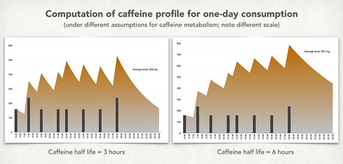
Putting the consumption and the initial condition into the equation and graphing it on a scale for the day in question we get

My average level was a bit high, but I'm used to it.

-- -- -- --
* I got this number from a doctor, but several sources have told me it's too low. Online sources point to a half-life of 3-6 hours. This changes the coefficient for $L(t-1)$ in the equation above to somewhere between 0.8909 (for three hours) to  0.9439 (for six hours). Possibly there's an update to this post in the future to deal with that.

Update in the future: I did the computations (click to embiggen):

Corrected Caffeine Level Profile

Sunday, July 17, 2016

Fun with numbers while walking

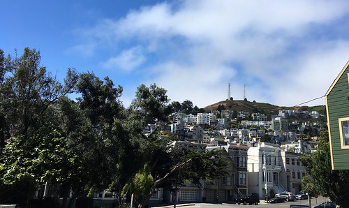
Walk in San Francisco, July 16, 2016


Yesterday I went for a walk in San Francisco. To pass the time and keep my mind off the Pokemon Go players making pedestrian traffic in Golden Gate Park hazardous, I decided to do a few approximate calculations about jet engines.

Let's say a jet engine used as a gas generator produces 22 000Lbs (= 10 000 kgf or 100 000 Newton, approximately) of thrust at a nozzle velocity of 720 km/h. How much air is it moving?

To generate thrust, a mass $m$ of air is accelerated from zero to 720 km/h (200 m/s) per second. The thrust is given by $F= ma$, so the flow, or mass/second, is 100 000/200 or 500kg/s. Since air density is about 1g/l at ground level, we need 500 cubic meters of air to go through the engine per second. That's the volume of a large room (20 by 10 meters surface, 2.5 meters ceiling) per second.

Just for fun, how much power is the engine generating? Considering only the kinetic energy imparted to the air (per second, since we're interested in power), we have $1/2 \times 500 \times (200)^2$, or 10  MW. Of course, since the air is very hot, some more power could be recovered using heat exchangers on the power turbine exhaust gases (making it a Brayton-Rankine combined cycle power plant).

Since a gas generator has an efficiency of around 1/3, this turbine will need about 30 megajoule of chemical energy per second entering the combustors, or about one liter of jet fuel every 1.2 seconds. (Looked up jet fuel energy density on my phone while walking --- ain’t living in the future grand? In the past I'd have to look that up in Perry's or Marks'.)

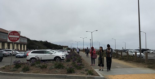
Yes, the numbers are very rough approximations; that's what you do when walking around. I also picked numbers that would be easy to divide in my head. Remember, I had to avoid Pokemon Go players who kept moving in unpredictable patterns in my path:

Walk in San Francisco, July 16, 2016


Edited (about 30 minutes after posting): During my walk I incorrectly computed the power as 1 MW instead of 10 MW, basically because keeping a lot of zeros in your head while avoiding the Pokemaniacs is difficult. The original post used that value; while rereading it after posting, I realized my order-of magnitude error and corrected it and the fuel calculation.

Sunday, July 10, 2016

Two lessons from a simple puzzle

Suppose you're given a set of fifteen integers for a puzzle:

$A = \{ 1, 3, 7, 11, 19, 23, 35, 37, 41, 43, 57, 59, 61, 67, 71\}.$

The puzzle is to add six of these numbers to make up $101$.

Take a moment to try to solve it.

Ready to proceed?

Before we get to the puzzle, one of the people along the chain that brought me this puzzle said that there were "hundreds of combinations."

True. There are indeed fifty "hundred combinations" (plus five), since $\left(15 \atop 6\right) = 5005$.

Apparently a number of children and adults had been searching for the solution and someone thought that writing a search program would be a good idea; they didn't know how to do it, though, since none of them were programmers. Personally, I'd do it in Prolog, since tree searches are so easy to program in it.

Except...

Except that all the numbers in $A$ are odd, as is $101$. And a sum of six odd numbers is necessarily an even number. The problem has no solution.
PROOF: Each number we pick, $n_i \in A$, is odd so it can be written as $n_i = 2 \times k_i +1$ for $k_i$ integer; adding six of them yields 
$2\times (k_1 + k_2 + k_3+ k_4+ k_5+ k_6) + 6$, 
which is even for any $k_i$.
Some of the adults involved were primary school teachers. Who teach basic arithmetic. And apparently not one of them abstracted from the numbers long enough to see that the problem was impossible. I'm told some of them didn't want to believe there was no solution.

So, here are two lessons from this simple puzzle:

1. Understanding beats blind search.

2. Statements of "impossible" require a proof.

Saturday, March 5, 2016

Powerlifters vs Gym Rats - A tale of two means

In my last post I wrote:

For example, some time ago I had a discussion with a friend about strength training. The gist of it was that powerlifters are typically much stronger than the average athlete, but they are also much fewer; because of that, in a typical gym the strongest athlete might not be a powerlifter, but as we get into regional competitions and national competitions, the winner is going to be a powerlifter.

And the explanation, which the friend didn't understand, was "because on the upper tail the difference between means is going to dominate the difference in sizes of the population."

So here's an illustration of what I meant, with pictures and numbers and bad jokes.

First let's make the setup explicit. That's the great power of math and numerical examples, making things explicit. "Powerlifters are typically much stronger than the average athlete" will be operationalized with four assumptions:
A1: There's some composite metric of strength, call it $S$ that we care about and we'll normalize it so that the average gym rat has a mean $\mu(S_{\mathrm{GR}})$ of zero and a variance of $1$. 
A2: The distribution of strength within the population of gym rats is Normally distributed. 
A3: The distribution of strength in the sub-population of powerlifters is also Normally distributed. 
A4: For illustration purposes only, we will assume that powerlifters have a mean $\mu(S_{\mathrm{PL}})$ of 2 and the same variance as the rest of the gym rats.
We operationalize "they are also much fewer" with
A5: For illustration, the number of powerlifters is $1\%$ of gym rats.
(Powerlifters are gym rats, so the distribution for $S_{\mathrm{GR}}$ includes these $1\%$, balanced by CrossFit people, who bring down the mean strength and IQ in the gym while raising the insurance premiums. Watch Elgintensity to understand.)

The following figure shows the distributions:


When we look at the people in a gym with above-average strength, that is people with $S_{\mathrm{GR}}>0$, we find that one-half of all gym rats have that, and $98
\%$ of all powerlifters have that: $\Pr(S_{\mathrm{GR}}>0) = 0.5$ and $\Pr(S_{\mathrm{PL}}>0) = 0.98$. This is illustrated in the next figure:


Powerlifters are over-represented in the above-average strength, approximately twice as much as in the general population, but they are only about $2\%$ of the total, as their over-representation is multiplied by $1\%$.

As we become more selective, the over-representation goes up. For athletes that are at least one standard deviation above the mean, we have:


with $\Pr(S_{\mathrm{GR}}>1) = 0.16$ and $\Pr(S_{\mathrm{PL}}>1) = 0.84$. Powerlifters are over-represented 5-fold, so about $5\%$ of the total athletes in this category.

When we become more and more selective, for example when we compute the number of gym rats that have at least as much strength as the average powerlifter, $\Pr(S_{\mathrm{GR}}>2)$, we get


with $\Pr(S_{\mathrm{GR}}>2) = 0.023$ and $\Pr(S_{\mathrm{PL}}>2) = 0.5$, a 22-fold over-representation, meaning that of every six athletes in this category, one is a powerlifter. (Yes, one out of six, not one out of five. See if you can figure out why; if not, look at the solution for $S>6$ below and you'll understand. Or not, but that's a different problem.)

And as we look at subsets of stronger and stronger athletes, the over-representation of powerlifters becomes higher and higher: $\Pr(S_{\mathrm{GR}}>3) = 0.00135$ and $\Pr(S_{\mathrm{PL}}>3) = 0.159$, $118$-fold ratio. There will be a few more powerlifters in this group that other gym rats; another way to say that is that powerlifters will be a little bit more than one-half of all gym rats that are at least one standard deviation stronger than the average powerlifter.

The ratios grow exponentially with increasing values for strength (the rare correct use of "exponentially" as they are ratios of Normal distribution tail probabilities; see below).

For $S>4$ the ratio is $718$, for $S>5$ the ratio is $4700$, for $S>6$ the ratio is $32 100$, in other words, there will be one non-powerlifter per group of $322$ gym rats with strength greater than 6 standard deviations above the mean of all gym rats.

This is what the effect of the differences in the tails of Normals always implies: eventually the small size of the better population (powerlifters) will be irrelevant as the higher mean will dominate.

See? That wasn't complicated at all.

-- -- -- --

For the mathematically inclined (strangely themselves over-represented in the set of powerlifters...)

Note that the ratio of probability density functions for the two Normal distributions in the post, for realizations of strength $S = x$ is
\[
\frac{f_{S}(x|\mu_{S}=2)}{f_{S}(x|\mu_{S}=0)}= \frac{e^{-(x-2)^2/2}}{e^{-x^2/2}}= e^{2x-2}
\]
which grows unbounded with $x$; no matter how small the fraction of powerlifters, say $\epsilon$, there's always a minimal $\bar S$ beyond which that ratio becomes greater than $1/\epsilon$ Which means that at some point above $\bar S$ the ratio of the remaining tail itself becomes greater than $1/\epsilon$. (It's very easy to calculate $\bar S$ and I have done so; I'll leave it as an exercise for the dedicated reader...)

Oh, that's the rare occurrence of the correct use of "exponentially," which is usually incorrectly treated as a synonym for "convex."

Wednesday, March 2, 2016

Acalculia, innumeracy, or numerophobia?

I think there's an epidemic of number-induced brain paralysis going around.

There are quite a few examples of quant questions in interviews creating the mental equivalent of a frozen operating system (including this post by Sprezzaturian), but I think that there's something beyond that, something that applies in social situations and that affects people who should know better.

Here's a simple example. What is the orbital speed of the International Space Station, roughly? No, don't google it, calculate it. Orbital period is about 90 minutes, altitude (distance to ground) about 400km, Earth radius is about 6370km.

Seriously, this question stumps people with university degrees, including some in the life sciences who necessarily have taken college level science courses.

And what college-level math do you need to answer it? The formula for the circumference of a circle of radius $r$. Yes, $2\times\pi\times r$. The orbital velocity in km/h is the total number of kilometers per orbit ($2\times\pi\times (6370+400)$) divided by the time to orbit in hours ($1\frac{1}{2}$), that is around $28\,000$ km/h, which is close to the actual value, $27\, 600$ km/h. (The orbit is an ellipse and takes more than 90 minutes.)

Can it possibly be ignorance, innumeracy? Is it plausible that college-educated professionals don't know the circumference formula?  Nope, they can recite the formula when prompted.

Or is it acalculia? That they have a mental inability to do calculation? Nope, they can compute exactly how much I owe on the lunch bill for the extra crème brûlée and the expensive entrée.

No, I think it's a mild case of numerophobia, a mental paralysis created by the appearance of an unexpected numerical challenge in normal life. This is a problem, as most of the world can be perceived more deeply if one thinks like a quant all the time; many strange "paradoxes" become obvious when seen through the lens of numerical (or parametrical) thinking.

For example, some time ago I had a discussion with a friend about strength training. The gist of it was that powerlifters are typically much stronger than the average athlete, but they are also much fewer; because of that, in a typical gym the strongest athlete might not be a powerlifter, but as we get into regional competitions and national competitions, the winner is going to be a powerlifter.

"That's because on the upper tail the difference between means is going to dominate the difference in sizes of the population." That quoted sentence is what I said. I might as well have said "boo-blee-gaa-gee in-a-gadda-vida hidee-hidee-hidee-oh" for all the comprehension. The friend is an engineer. A numbers person. But apparently, numbers are work-domain only.

The awesome power of quant thinking is being blocked by this strange social numerophobia. We must fight it. Liberate your inner quant; learn to love numbers in all areas of life.

Everything is numbers.

Sunday, January 24, 2016

Big numbers, big confusion; small numbers, bigger confusion.

I can make something almost impossible happen. And so can you.

Let's start by defining what "almost impossible" means. Less than one-in-a-trillion chance? How about less than one in a trillion-trillion chance? One in a trillion-trillion-trillion chance?

Ok, lets take a breath here. What's this trillion-trillion and trillion-etc stuff?

(In my observation, economists say million, billion, trillion, and all their audiences hear is "big number." Innumeracy over scale has bad consequences when applied to public policy.)

One trillion is 1,000,000,000,000. (Yes, I'm using American billions, pretty much like everyone else now does.) This is written as $10^{12}$. A trillion trillion is $10^{12} \times 10^{12} = 10^{24}$ and a trillion-trillion-trillion is $10^{36}$, a one followed by thirty-six zeros.

To put that number in perspective, the age of the Earth is about $4.5$ billion years, or about $1.42 \times 10^{17}$ seconds. That's 142,000 trillion seconds. Note that this is much smaller than a trillion-trillion seconds (it's over one seven-millionth of a trillion-trillion), let alone a trillion-trillion-trillion. If you had seven million planets the same age as the Earth, and you picked at random one specific second in the history in one specific planet you'd would have about a one in a trillion-trillion chance of picking this precise second on this planet. A one in a trillion-trillion-trillion chance is one trillion times smaller than that.

So, something that has a one in a trillion-trillion-trillion chance of happening has to be a very low probability event. Shall we call anything less likely than that "almost impossible"? We shall.

So, here's how I make something almost impossible happen, over and over again, and you can too: shuffle a deck of cards.

Using only 52 cards (no jokers), there are $52! = 52\times 51 \times \ldots \times 2$ possible card shuffles, and $52! \approx 8.1 \times 10^{67}$. That number is $8.1\times 10^{31}$ times bigger than a trillion-trillion-trillion.

And yet, every card shuffle produces an event with 1-in-$8.1 \times 10^{67}$ probability. You and I can generate scores of these "almost impossible" events using a simple deck of cards.

(A little thinking will lead an attentive reader to the solution to this apparent paradox. It's not a paradox. I will post a solution here in a few days, if I remember :-)

-- -- -- --

Just for fun, a simple brain teaser:

Imagine you have two decks of 52 cards (blue and red); what has more possible combinations, shuffling the two decks together and dividing into two piles of 52 cards by separating in the middle of the full shuffled two decks, or shuffling the two decks separately each into its pile?

(Yes, it's obvious for anyone conversant with combinatorics, but apparently not everyone is conversant with combinatorics. Common answer: "it's the same.")

Monday, November 26, 2012

How misleading "expected value" can be


The expression "expected value" can be highly misleading.

I was just writing some research results and used the expression "expected value" in relation to a discrete random walk of the form

$x[n+1] = \left\{ \begin{array}{ll}
   x[n] + 1 & \qquad \text{with prob. } 1/2 \\
  & \\
   x[n] -1 & \qquad \text{with prob. } 1/2
   \end{array}\right. $ .

This random walk is a martingale, so

$E\big[x[n+1]\big|x[n]\big] = x[n]$.

But from the above formula it's clear that it's never the case that $x[n+1] = x[n]$. Therefore, saying that $x[n+1]$'s expected value is $x[n]$ is misleading — in the sense that a large number of people may expect the event $x[n+1] = x[n]$ to occur rather frequently.

Mathematical language may share words with daily usage, but the meaning can be very different.

----

Added Nov 27: In the random walk above, for any odd $k$, $x[n+k] \neq x[n]$. On the other hand, here's an example of a martingale where $x[n+1] = x[n]$ happens with probability $p$, just for illustration:


$x[n+1] = \left\{ \begin{array}{ll}
   x[n] + 1 & \qquad \text{with prob. } (1-p)/2 \\

  & \\
   x[n]  & \qquad \text{with prob. } p \\

  & \\
   x[n] -1 & \qquad \text{with prob. } (1-p)/2
   \end{array}\right. $ .

(Someone asked if it was possible to have such a martingale, which makes me fear for the future of the world. Also, I'm clearly going for popular appeal in this blog...)

Friday, October 19, 2012

Math in business courses: derivating + grokking


I used to start my Product Management class with a couple of business math problems like the following: let's say we use a given market research technique to measure the value of a product; call the product $i$ and the value $v(i)$. We know -- by choice of the technique -- that the probability that the customer will buy $i$ is given by

$\Pr(i) = \frac{\exp(v(i))}{1 + \exp(v(i))}$.

My question: is this an increasing or a decreasing function of the $v(i)$?

Typically this exercise divided students in three groups:

First, students who were afraid of math, were looking for easy credits, or otherwise unprepared for the work in the class. These math problems made sure students knew what they were getting into.

Second, students who could do the math, either by plug-and-chug (take derivative, check the sign) or by noticing that the formula may be written as

$\Pr(i) = \frac{1}{1 + \exp(-v(i))}$

and working the increasing/decreasing chain rule.

Third, students who had a quasi-intuitive understanding ("grok" in Heinlein's word) that probability of purchase must be an increasing function of value, otherwise these words are being misused.

Ideally we should be training business students to mix the skills of the last two groups: a fluency in basic mathematical thinking and grokking business implications.

- - - - - - -

Administrative note: Since I keep writing 4000+ word drafts for "important" posts that never see the light of blog (may see the light of Kindle single), I've decided to start posting these bite-sized thoughts.

Thursday, January 19, 2012

A tale of two long tails

Power law (Zipf) long tails versus exponential (Poisson) long tails: mathematical musings with important real-world implications.

There's a lot of talk about long tails, both in finance (where fat tails, a/k/a kurtosis, turn hedging strategies into a false sense of safety) and in retail (where some people think they just invented niche marketing). I leave finance for people with better salaries brainpower, and focus only on retail for my examples.

A lot of money can be made serving the customers on the long tail; that much we already knew from decades of niche marketing. The question is how much, and for this there are quite a few considerations; I will focus on the difference between exponential decay (Poisson) long tails and hyperbolic decay (power law) long tails and how that difference would impact different emphasis on long tail targeting (that is, how much to invest going after these niche customers), say for a bookstore.

A Poisson distribution over $N\ge 0$ with parameter $\lambda$ has pdf:

$ \Pr(N=n|\lambda) =\frac{\lambda^{n}\, e^{-\lambda}}{n!}$.

A discrete power law (Zipf) distribution for $N\ge 1$ with parameter $s$ is given by:

$ \Pr(N=n|s) =\frac{n^{-s}}{\zeta(s)},$

where $\zeta(s)$ is the Riemann zeta function; note that it's only a scaling factor given $s$.

A couple of observations:

1. Because the power law has $\Pr(N=0|s)=0$, I'll actually use a Poisson + 1 process for the exponential long tail. This essentially means that the analysis would be restricted to people who buy at least one book. This assumption is not as bad as it might seem: (a) for brick-and-mortar retailers, this data is only collected when there's an actual purchase; (b) the process of buying a book at all -- which includes going to the store -- may be different from the process of deciding whether to buy a given book or the number of books to buy.

2. Since I'm not calibrating the parameters of these distributions on client data (which is confidential), I'm going to set these parameters to equalize the means of the two long tails. There are other approaches, for example setting them to minimize a measure of distance, say the Kullback-Leibler divergence or the mean square error, but the equal means is simpler.

The following diagram compares a Zipf distribution with $s=3$ (which makes $\mu=1.37$) and a 1 + Poisson process with $\lambda=0.37$ (click for larger):

Long tails example for blog post

The important data is the grey line, which maps into the right-side logarithmic scale: for all the visually impressive differences in the small numbers $N$ on the left, the really large ratios happen in the long tail. This is one of the issues a lot of probabilists point out to practitioners: it's really important to understand the behavior at the small probability areas of the distribution support, especially if they represent -- say -- the possibility of catastrophic losses in finance or the potential for the customers who buy large numbers of books.

An aside, from Seth Godin, about the importance of the heavy user segment in bookstores:

Amazon and the Kindle have killed the bookstore. Why? Because people who buy 100 or 300 books a year are gone forever. The typical American buys just one book a year for pleasure. Those people are meaningless to a bookstore. It's the heavy users that matter, and now officially, as 2009 ends, they have abandoned the bookstore. It's over.

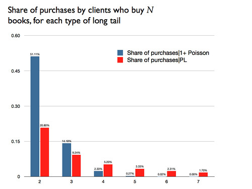
To illustrate the importance of even the relatively small ratios for a few books, this diagram shows the percentage of purchases categorized by size of purchase:

Long tails example for blog post

Yes, the large number of customers who buy a small number of books still gets a large percent of the total, but each of these is not a good customer to have: elaborating on Seth's post, these one-book customers are costly to serve, typically will buy a heavily-discounted best-seller and are unlikely to buy the high-margin specialized books, and tend to be followers, not influencers of what other customers will spend money on (so there are no spillovers from their purchase).

The small probabilities have been ignored long enough; finance is now becoming weary of kurtosis, marketing should go back to its roots and merge niche marketing with big data, instead of trying to reinvent the well-know wheel.

Lunchtime addendum: The differences between the exponential and the power law long tail are reproduced, to a smaller extent, across different power law regimes:

Comparing Power Law Regimes (for blog post)

Note that the logarithmic scale implies that the increasing vertical distances with $N$ are in fact increasing probability ratios.

- - - - - - - - -

Well, that plan to make this blog more popular really panned out, didn't it? :-)

Monday, December 12, 2011

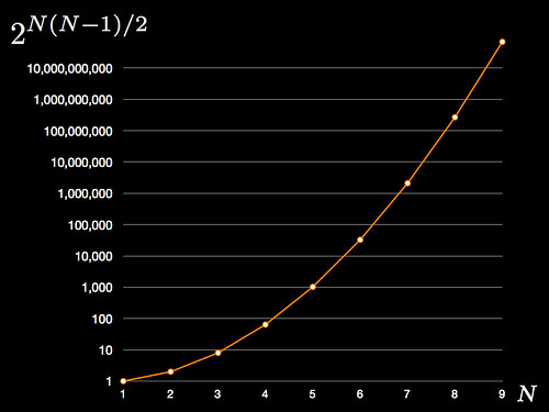
How many possible topologies can a N-node network have?

Short answer, for an undirected network: $2^{N(N-1)/2}$.

Essentially the number of edges is $N(N-1)/2$ so the number of possible topologies is two raised to the number of edges, capturing every possible case where an edge can either be present or absent. For a directed network the number of edges is twice that of those in an undirected network so the number of possible topologies is the square (or just remove the $/2$ part from the formula above).

To show how quickly things get out of control, here are some numbers:

$N=1 \Rightarrow 1$ topology
$N=2 \Rightarrow 2$ topologies
$N=3 \Rightarrow 8$ topologies
$N=4 \Rightarrow 64$ topologies
$N=5 \Rightarrow 1024$ topologies
$N=6 \Rightarrow 32,768$ topologies
$N=7 \Rightarrow 2,097,152$ topologies
$N=8 \Rightarrow 268,435,456$ topologies
$N=9 \Rightarrow 68,719,476,736$ topologies
$N=10 \Rightarrow 35,184,372,088,832$ topologies
$N=20 \Rightarrow 1.5693 \times 10^{57}$ topologies
$N=30 \Rightarrow 8.8725 \times 10^{130}$ topologies
$N=40 \Rightarrow 6.3591 \times 10^{234}$ topologies
$N=50 \Rightarrow 5.7776 \times 10^{368}$ topologies

This is the reason why any serious analysis of a network requires the use of mathematical modeling and computer processing: our human brains are not equipped to deal with this kind of exploding complexity.

And for the visual learners, here's a graph denoting the pointlessness of trying to grasp network topologies "by hand" (note logarithmic vertical scale):

Number of network topologies as a function of the number of nodes

Sunday, November 13, 2011

Vanity Fair bungles probability example

There's an interesting article about Danny Kahneman in Vanity Fair, written by Michael Lewis. Kahneman's book Thinking: Fast And Slow is an interesting review of the state of decision psychology and well worth reading, as it the Vanity Fair article.

But the quiz attached to that article is an example of how not to popularize technical content.

This example, question 2, is wrong:
A team of psychologists performed personality tests on 100 professionals, of which 30 were engineers and 70 were lawyers. Brief descriptions were written for each subject. The following is a sample of one of the resulting descriptions:


Jack is a 45-year-old man. He is married and has four children. He is generally conservative, careful, and ambitious. He shows no interest in political and social issues and spends most of his free time on his many hobbies, which include home carpentry, sailing, and mathematics. 
What is the probability that Jack is one of the 30 engineers?


A. 10–40 percent
B. 40–60 percent
C. 60–80 percent
D. 80–100 percent


If you answered anything but A (the correct response being precisely 30 percent), you have fallen victim to the representativeness heuristic again, despite having just read about it. 
No. Most people have knowledge beyond what is in the description; so, starting from the appropriate prior probabilities, $p(law) = 0.7$ and $p(eng) = 0.3$, they update them with the fact that engineers like math more than lawyers, $p(math|eng) >> p(math|law)$. For illustration consider

$p(math|eng) = 0.5$; half the engineers have math as a hobby.
$p(math|law) = 0.001$; one in a thousand lawyers has math as a hobby.

Then the posterior probabilities (once the description is known) are given by
$p(eng|math) = \frac{ p(math|eng) \times p(eng)}{p(math)}$
$p(law|math) = \frac{ p(math|law) \times p(law)}{p(math)}$
with $p(math) = p(math|eng) \times p(eng) + p(math|law) \times p(law)$. In other words, with the conditional probabilities above,
$p(eng|math) = 0.995$
$p(law|math) = 0.005$
Note that even if engineers as a rule don't like math, only a small minority does, the probability is still much higher than 0.30 as long as the minority of engineers is larger than the minority of lawyers*:
$p(math|eng) = 0.25$ implies $p(eng|math) = 0.991$
$p(math|eng) = 0.10$ implies $p(eng|math) = 0.977$
$p(math|eng) = 0.05$ implies $p(eng|math) = 0.955$
$p(math|eng) = 0.01$ implies $p(eng|math) = 0.811$
$p(math|eng) = 0.005$ implies $p(eng|math) = 0.682$
$p(math|eng) = 0.002$ implies $p(eng|math) = 0.462$
Yes, that last case is a two-to-one ratio of engineers who like math to lawyers who like math; and it still falls out of the 10-40pct category.

I understand the representativeness heuristic, which mistakes $p(math|eng)/p(math|law)$ for $p(eng|math)/p(law|math)$, ignoring the base rates, but there's no reason to give up the inference process if some data in the description is actually informative.

-- -- -- --
* This example shows the elucidative power of working through some numbers. One might be tempted to say "ok, there's some updating, but it will probably still fall under the 10-40pct category" or "you may get large numbers with a disproportionate example like one-half of the engineers and one-in-a-thousand lawyers, but that's just an extreme case." Once we get some numbers down, these two arguments fail miserably.

Numbers are like examples, personas, and prototypes: they force assumptions and definitions out in the open.

Sunday, September 18, 2011

Probability interlude: from discrete events to continuous time

Lunchtime fun: the relationship between Bernoulli and Exponential distributions.

Let's say the probability of Joe getting a coupon for Pepsi in any given time interval $\Delta t$, say a month, is given by $p$. This probability depends on a number of things, such as intensity of couponing activity, quality of targeting, Joe not throwing away all junk mail, etc.

For a given integer number of months, $n$, we can easily compute the probability, $P$, of Joe getting at least one coupon during the period, which we'll call $t$, as

$P(n) = 1 - (1-p)^n$.

Since the period $t$  is $t= n \times \Delta t$, we can write that as

$P(t) = 1 - (1-p)^{\frac{t}{\Delta t}}.$

Or, with a bunch of assumptions that we'll assume away,

$P(t) = 1- \exp\left(t \times \frac{\log (1-p)}{\Delta t}\right).$

Note that $\log (1-p)<0$. Defining $r = - \log (1-p) /\Delta t$, we get

$P(t) = 1 - \exp (- r t)$.

And that is the relationship between the Bernoulli distribution and the Exponential distribution.

We can now build continuous-time analyses of couponing activity. Continuous analysis is much easier to do than discrete analysis. Also, though most simulators are, by computational necessity, discrete, building them based on continuous time models is usually simpler and easier to explain to managers using them.