A common misconception about scale effects (for example, in production functions)

There's a common misperception that if a function (usually a production function or a consumer valuation function) scales proportionally (meaning that when all inputs double, for example, the output doubles), then that function must be a linear function.

Sadly, some of the people falling for this error make important decisions in market research and in capacity planning, two areas where this kind of behavior (scaling proportionally) happens a lot and where the error in considering only linear models may have serious consequences for the bottom line.

(And we should always strive to make fewer math errors, of course.)

Let's start with the simple part, using a two-variable function:

\[  f(x,y) = a \, x + b \, y \]

If we scale $x$ and $y$ by a constant $c$ we get

\[ f(cx,cy) = a \, cx + b \, cy = c (a \, x + b \, y) = c \, f(x,y).\]

Clearly, linear functions scale proportionately. What about the other part, the ``must be a linear function'' part?

That's wrong. And we need no more than an example to show it. Voilá:

\[ f(x,y) = x^\alpha \, y^{(1-\alpha)}\]

for an $\alpha \in (0,1)$.

That function is not linear at all; here's a plot for $\alpha = 0.5$ and $x,y$ each in $[0,10]$ (that makes the $z = f(x,y)$ variable also in $[0,10]$, obviously):

And yet,

\[ f(cx,cy) = (cx)^\alpha \, (cy)^{(1-\alpha)} = c^{\alpha + (1-\alpha)} \, x^\alpha \, y^{(1-\alpha)} = c  f(x,y). \]

So, now we know not to limit ourselves to linear functions when describing systems that exhibit proportional scaling.

Nerd note: a function that scales proportionally is called ``homothetic'' or ``homogeneous of degree one.''

We don't need fraud to get a replication crisis

(A longer version of this is going in the technical notes for my book, so there are references here to it.)

We can use an analysis like the one in [book chapter] to understand the so-called ``replication crisis,'' of many research papers failing to replicate.

We'll sidestep the controversies about suspicion of fraud in specific results and show how the same random clusters that happen in car crashes and diseases can lead to this replication crisis (i.e. they create positive results with data that doesn't show them).

(Some authors of the papers that failed to replicate have admitted to various levels of fraud and several papers have been retracted due to strong indications of fraud. We're not disputing that fraud exists. But here we show that large numbers of well-intentioned researchers in a field, combined with a publication bias towards positive results, can generate false results just by probability alone.)

As we saw in the Statistics Are Weird Interlude, when using a sample to make judgments about the population, a traditional (frequentist) way to express confidence in the results is by testing them and reporting a confidence level. For historical reasons many fields accept 95% as that confidence level.

Reminder: The general public assumes that 95% confidence level means that the phenomenon is true with probability $0.95$, given the test results. That's not how it works: the 95% confidence means that the probability that we get the test result when the phenomenon is true is $0.95$. In other words, the public perception is a probability of the truth of the phenomenon conditional on the result of the test, the real meaning is a probability of the result conditioned on the truth of the phenomenon, and in general

\[ \text{[perception] } \Pr(\text{phenomenon}|\text{result}) \neq \Pr(\text{result}|\text{phenomenon}) \text{ [reality]}\]

There's a schism in statistics about whether and how to use uninformative priors and chained Bayes rule ---as described in the Bayesian Interlude--- to deal with multiple experiments (the frequentists' approach being ``not to use them at all''). We'll sidestep those discussions here, but point out their implications further down. End of reminder.

So, the probability that we get a false positive from testing a data set for a non-existent phenomenon at the 95% confidence level is $p \le 0.05$ and we'll use the equal value for our modeling, $p = 0.05$.

Let's say we have a team of scientists investigating the very important phenomenon of whether liking pineapple on pizza makes a person more likely to put real cream, rather than non-dairy creamer, in their coffee.

To investigate this important matter, the team chooses a sample of the population and runs some controlled experiment. Maybe the result is positive, or maybe it's negative; but since they have funding, the scientists can run more experiments, controlling for different variables (is the pizza deep-dish? do people put honey or sugar in the coffee with their cream/creamer? these are called covariates or, sometimes, controls). Say the team runs 100 experiments in total.

Now we make our important assumption, which we can do because we always play in God-mode: in reality there's no relationship between pineapple on pizza and the choice of cream or creamer in coffee.*

Because of that assumption, all the positives in the data will be false positives, and we know that those happen with $p = 0.05$, by our setup. So, in 100 experiments there should be an average of 5 false positives, and the number of false positives itself is a random variable, say $N$, distributed Poisson with parameter 5. The next figure shows that distribution.

We can also ask some simple questions: how likely is the team to observe at least, say 7 positive results? How about 10? These are easily calculated:

\[ \Pr(N\ge 7) = 1-F_N(6) = 0.24 \quad\text{and}\quad \Pr(N\ge 10) = 1-F_N(9) = 0.03.\]

So, in almost one-quarter of the parallel universes that people use to interpret probabilities as frequencies there'll be seven or more positive results, but only in 3% there'll be ten or more.

This may look like cherry-picking of experiments, but it's very easy for a well-meaning team to come up with reasons why an experiment that failed to produce the desired result had a design flaw. Whereas the usual form of cherry-picking, selecting the data points within an experiment, is generally recognized by all researchers as fraud.**

But wait, there's more…

Important scientific questions like the relationship of pineapple on pizza to real cream in coffee attract large numbers of people to scientific research; so there are other teams investigating this important phenomenon. When we consider that, we can ask how likely it is for us to see a paper with 7, 8, 9, or even 10 positive results, given a total number of teams $T$ investigating this question.

The next figure shows the probability of at least one team in $T$ finding at least $N$ positive results at a 95% certainty level when each team runs 100 experiments; remember that this is given that there's no phenomenon.

With 10 teams there's a 50:50 chance of a team finding 9 or more positive results. That's usually considered a very high level of cross validation (each experiment validating and being validated by at least 8 others). And it's all based on a non-existent phenomenon.

Because scientific publications (and the mass media) tend to publish only positive results (results that show something different from what was expected), this publication bias together with the large numbers of teams $T$ and repeated experiments (here we used 100 experiments per team) can create the illusion of phenomena where none exist. Later, when these phenomena are assumed to be the default position, other researchers find them to be non-existent, and the replication crisis that we're seeing now ensues.

It's not a replication crisis, it's a ``too many phenomena were artifacts'' crisis.***

- - - -

* As this is a blog post and not the book or technical notes, here are my opinions on these weighty matters: pineapple on pizza, yes (but no pizza in the P:E diet, so it's a moot point); creamer, cream, honey, sugar, syrups, or any other adulterants in coffee, Heck no! 

** Note how the Bayesian approach deals with chains of experiments and non/low-informative results: the probability of the phenomenon given the result, $\Pr(P|R)$, given by Bayes's rule is

\[\Pr(P|R) = \frac{\Pr(R|P) \, \Pr(P)}{\Pr(R)}.\]

Bayesians can easily integrate new results with previous experiments by using the $\Pr(P)$, therefore chaining inference instead of disposing of experiments that "didn't work." And a low-informative result, where $\Pr(R|P) \simeq \Pr(R)$, i.e. the result happens with almost the same probability whether or not the phenomenon is true, will be automatically accounted as such by making $\Pr(P|R) \simeq \Pr(P)$, in other words negating its effect without disposing of its data as cherry-picking would.

*** Granted, there was some fraud as well.

A thought about the DANMASK study and presenting quantitative results

This post is about the analysis and presentation of the results, not about the substantive question of whether to wear masks. Link to the study. 

The main point here is that the way the results are presented, without a comparison counterfactual, makes it difficult to understand what the study really means:

So, without further ado, the results themselves. Cutting through a lot of important but uninteresting stuff, there are four numbers that matter:

Size of the sub-sample with masks: 2392

Number of infected in the mask sub-sample: 43

Size of the sub-sample with no masks: 2470

Number of infected in the no-mask sub-sample: 52

From these four numbers we can compute the incidence of infection given masks (1.8%) and no masks (2.1%). We can also test these numbers in a variety of ways, including using the disaggregate data to calibrate a logit model (no, I won't call it ``logistic regression''), but for now let's look at those two incidences only.

A likelihood ratio "test"

Here's a simple test we like: the likelihood ratio test between two hypotheses: that both samples are drawn from a common incidence (1.95%) or that each sample is drawn from its own incidence. In other words, we want

\[ LR = \frac{\Pr(52 \text{ pos out of } 2470|p = 0.021)\, \Pr(43 \text{ pos out of } 2392|p = 0.018)}{\Pr(52 \text{ pos out of } 2470|p = 0.0195)\, \Pr(43 \text{ pos out of } 2392|p = 0.0195)}\]

Using log-space computations to get around precision problems, we get $LR = 1.083$.

In other words, it's only 8.3% more likely that the data comes from two groups with different incidences than from a group with a common incidence. In order to be minimally convinced we'd like that likelihood ratio to be 20 or so, at least, so LR = 1.083 supports the frequentist analysis that these numbers seem to come from the same population.

(Yes, this is the same test we apply to Rotten Tomatoes ratings.)

Presenting the results: make comparisons!

A problem with the paper is that the academese of the results is hard for many people to understand. One way to make the lack of effect of masks more obvious is to create a comparison with an alternative. We choose a simple 2:1 ratio of protection, which is weak protection (a person wearing a mask has half the likelihood of infection of that of someone with no mask), but is enough to make the point.

Since we want to make fair comparison, we need to use the same size population for both the mask and no-mask conditions (we'll choose 2400 as it's in the middle of those sample sizes) and infection ratios similar to those of the test (we choose 1.25% and 2.5% for mask and no-mask, respectively). Now all we need to do is plot and compare:

(The more eagle-eyed readers will notice that these are Poisson distributions.)

The comparison with an hypothetical, even one as basic as a 2:1 protection ratio makes the point that the distributions on the left overlap a lot and therefore there's a fair chance that they come from the same population (in other words that there's no difference in incidence of infections between the use and non-use of masks).

Bayesians (and more attentive frequentists) might note at this point that having non-significant differences isn't the same thing as having a zero effect size; and that a richer model (including the distributions of the estimates themselves, which are random variables) might be useful to drive policy.

But for now, the point is that those four lines in the figure are much easier to interpret than the word-and-number salad under the subheading "results" in the paper itself.

Why is it so hard for people to change their minds?

The usual explanation is that people discount information that contradicts their beliefs. Let's build a model to explore this idea. 

We analyze the evolution of beliefs of a decision-maker receiving outside information, and to start we'll assume that the decision-maker is rational in the Bayesian sense, i.e. uses Bayes's rule with the correct conditional probabilities to update beliefs.

We call the variable of interest $X$ and it's binary: true/false, 1/0, red/blue. For the purposes of this discussion $X$ could be the existence of water on Pluto or whether the New England Patriots deflate their footballs. 

There's a true $X \in \{0,1\}$ out there, but the decision-maker doesn't know it. We will denote the probability of $X=1$ by $p$, and since there's information coming in, we index it: $p[n]$ is the probability that $X=1$ given $n$ pieces of information $X_1 \ldots X_n$.

We start with $p[0] = 1/2$, as the decision-maker doesn't know anything. A piece of information $X_i$ comes in, with reliability $r_i$, defined as $\Pr(X_i = X) = r_i$; in other words false positives and false negatives have the same probability, $(1-r_i)$.

Using Bayes's rule to update information, we have

$p[i] = \frac{r_i \, p[i-1]}{r_i \, p[i-1] + (1-r_i)(1-p[i-1])}$, if $X_i = 1$ and

$p[i] = \frac{(1-r_i) \, p[i-1]}{r_i \, (1-p[i-1]) + (1-r_i) \, p[i-1]}$, if $X_i = 0$.

For illustration, let's have the true $X=1$ (so there's indeed water in Pluto and/or the Patriots do deflate their balls), and $r_i = r$, fixed for all $i$; with these definitions, $\Pr(X_i = 1) = r$. We can now iterate $p[i]$ using some random draws for $X_i$ consistent with the $r$; here are some simulations of the path of $p[i]$, three each for $r = 0.6, 0.7, 0.8$.*

Essentially, truth wins out eventually. The more reliable the information, the faster the convergence. So, that whole "it's easier to fool someone than to get them to realize they were fooled" was wrong, wasn't it?

Only if people are Bayesian updaters with accurate perception of the reliability. In particular, when they don't let their beliefs bias that perception.

Huh-Oh!

Let us consider the case of biased perception. The simplest approach is to consider that the decision-maker's perception of reliability depends on whether the $X_i$ is in support or against current beliefs.

For simplicity the true reliability of information will still be a constant, denoted $r$; but the decision maker uses a $r_i$ that is dependent on the $X_i$ and the $p[i-1]$: if they agree (for example $p[i-1]>1/2$ and $X_i = 1$),  then $r_i = r$; if they don't (for example $p[i-1]<1/2$ and $X_i = 1$), then $r_i = (1-r)$.

Note that the $X_i$ are still generated by a process that has $\Pr(X_i = 1) = r$, but now the decision-maker's beliefs are updated using the $r_i$, which are only correct  ($r_i = r$) for draws of $X_i$ that are consistent with the beliefs $p[i-1]$, and are precisely opposite ($r_i = 1-r$) otherwise.

To illustrate this biased behavior, in the following charts we force $X_1 = 0$ (recall that $X=1$), so that the decision-maker starts with the wrong information.

There are just a few of the many paths, but they illustrate three elements that tended to be common across most simulations:

1. There's a lot more volatility in the beliefs, and much slower convergence. Sometimes, like the middle case with $r=0.8$, there's a complete flip from $p[i] \simeq 0$ to a quick convergence to the true $p[i] \simeq 1$; this was rare but worth showing one example in the image.
2. There are many cases when the decision-maker stays very close to the wrong $p[i]\simeq 0$ for very long periods (sometimes for the total length of the simulation, 1000 steps; the graphs are for the first 60 because that was enough for illustration).
3. The higher the reliability the more volatile the results can be, unlike in the case with fixed $r_i$. In general increasing reliability $r$ didn't help much with convergence or stability.

So, when people start biasing their perspectives (which might come from changing the reliability, what was simulated here, or from ignoring information that contradicts their beliefs, which is similar in effect), to counter the effect of bad early information (the $X_1 = 0$) it takes a lot of counteracting new information.

Lucky for us, people in the real world don't have these biases, they're all perfect Bayesians. Otherwise, things could get ugly.

😉

- - - - 

* In case it's not obvious, the effect of $r_i$ is symmetric around 0.5: because of how the information is integrated, the patterns for $r=0.6$ and $r=0.4$ are identical. As a consequence, when $r=0.5$ there's no learning at all and the decision-maker never moves away from $p = 0.5$.

OBSERVATION: There are also strategic and signaling reasons why people don't publicly change their minds, because that can be used against them by other players in competitive situations; but that's a more complicated — and to some extent trivial, because obvious in hindsight — situation, since it involves the incentives of many decision-makers and raises questions of mechanism design.

Why can't we have civil discussions?

Partly, or mostly, because some people profit handsomely from the lack of civil discourse, and their audiences, to a large extent, like the demonizing of the opposition.

Monetizing the echo chamber versus persuading the opposition

To illustrate these two approaches to being a public intellectual [broadly defined], consider the difference between Carl Sagan and Person 2, both of whom were not fans of religion:

Here's how the TV series Cosmos starts:

[Vangelis music plays] Carl Sagan: The Cosmos is all there is, there ever was, or there ever will be. [...] The size and age of the Cosmos are beyond normal human understanding. Lost somewhere between immensity and eternity is our tiny planetary home, the Earth. [...] In the last few Millennia we've made astonishing discoveries about the Cosmos and our place in it.

Person 2 [who will remain anonymous] wrote the following in a book :

The God of the Old Testament is arguably the most unpleasant character in all fiction: jealous and proud of it; a petty, unjust, unforgiving control-freak; a vindictive, bloodthirsty ethnic cleanser; a misogynistic, homophobic, racist, infanticidal, genocidal, filicidal, pestilential, megalomaniacal, sado-masochistic, capriciously malevolent bully.

Carl Sagan welcomed all into his personal voyage (the subtitle of the Cosmos show) to explore the Cosmos. Sagan's approach was a non-confrontational way to make religious people question, for example, young-Earth creationism. Sagan was persuading the opposition.

Person 2 wrote books (and gave speeches and appeared on television programs) to make his audience feel superior to the religious, just for not being religious; this is what is called monetizing the echo chamber.

Some public intellectuals are more interested in monetizing their echo chamber than in persuading the opposition. This has dire consequences for public discourse: it aggravates divisions, demonizes positions and people, and makes cooperation difficult across party lines.

But it appeals to some of the darker parts of human nature and is easier than persuading the opposition, so a lot of people seem to prefer it (both speakers/authors and audiences). And since it tends to demonize the opposition, it also gives that opposition both incentives and material to respond in the same fashion.

In other words, it's a self-reinforcing mechanism and one that makes us all worse-off in the long term, as divisions and demonizations aren't conducive to civil and productive societies.

A simple model of this behavior

Let's define the neutral position (as in we don't badmouth anyone and stick to the science) as the zero point in some scale, and consider the evolution of the discourse by two opposing factions, $A$ and $B$. Movement away from the zero means that these factions are more and more focused on monetizing their echo chamber rather than convincing those who may be neutral or even believe in the opposite position.

We model the evolution of the discourse by a discrete stochastic process (i.e. the positions change with time but there are some random events that affect their movement). Each side has a drift $D$ in the direction of their position and also a tendency to respond to the other side's positions. To model this response, we'll use a tit-for-tat approach, in which the response at a given time is proportional to what the other side's position was in the previous time. In other words, we have the following dynamics:

$A[i+1] = A[i] + D  - S \times B[i] + \epsilon_{Ai} \qquad\text{with } \epsilon_{Ai} \sim \mathrm{N}(0, \sigma)$

and 

$B[i+1] = B[i] – D  - S \times A[i] + \epsilon_{Bi}  \qquad\text{with }  \epsilon_{Bi} \sim \mathrm{N}(0, \sigma)$

With this formulation $A$ tends to drift to positive values and $B$ tends to drift to negative values, assuming that $D$ is positive. The following figure shows how the dynamics evolve for some values of these $D$ and $S$ parameters

Note how in all cases we have divergence from zero (i.e. monetizing of the echo chamber, to the exclusion of persuading the opposition) and in particular how the increase in tit-for-tat sensitivity leads to acceleration of this process.

(The point of making a model like this [a theoretical model] is to see what happens when we change the parameters. I recommend readers make their own versions to play around with; mine were made in the R programming language on Rstudio and Tuftized/prettified for display on Apple Keynote, but it's easy enough to set that model up in a spreadsheet.) 

What can we do?

Since this is a systemic problem (a problem composed of large scale incentives and human nature), there's little that can be done with individual actions, but there are a few good starting points:

1. Avoid giving attention (much less money) to people who are monetizing the echo chamber, that is people who are deliberately making out discourse less civil for profit.
2. Focus on positives rather than negatives: despite the popularity of Person 2, there are plenty of science popularizers who focus, as Carl Sagan did, on the majesty of the Universe and the power of science and technology.
3. Point out this difference, between monetizers of the echo chamber and persuaders of the opposition, to other people, so that they too can start focussing on the positive
4. Reflect on what we do, ourselves: do we focus on the negative or the positive? (This led to a lot fewer tweets on my part as I either stop snarky responses before I tweet or delete them soon after realizing they aren't helping.)*

- - - -

* Note that pointing out a technical or modeling error is not covered by this: if someone says 2+2=5, the right thing is not to make fun of them for it, but rather correct them. However, ignoring the error is not positive; the error must be corrected, though the person making it need not be demonized (it's counterproductive to demonize people who are wrong, as that leads to defensiveness). Carl Sagan in the example above repeatedly undermines young-Earth creationism without ever mentioning it. 

ORIGIN: This post was motivated by a video on the Covid-19 situation by a person with whom I would agree about 95% on substance. But that video was such a collection of out-group demonizing and in-group pandering that it did change one mind: mine. Not about the substantive matters, but about subscribing to or otherwise following the social media of people whose entire schtick is monetizing their echo chamber.

Pomposity!

Let $f(x)$, $f \in \mathrm{C}^{\infty}$, be the following infinitely continuously differentiable function over the space of real numbers:

\[ 
f(x) \doteq 
\sum_{n=0}^{\infty} \frac{e^{-2} \, 2^n}{n!}
+ \frac{1}{\sqrt{2 \, \pi}}\int_{-\infty}^{+ \infty} x  \, \exp(-y^2/2) \, dy;
\]
then, applying Taylor's theorem and the Newton–Leibniz axiom,

\[f(1) = 2.\]

Time out! What the Heck?!?!

Okay. Breathe.

Let's restate the above in non-pompous terms.

Let $f(x)$ be the following function
\[f(x) = 1 + x\]
then $f(1) = 2$.

All the words between "following" and "function" in the first paragraph mean "smooth," which this function certainly is; $f \in \mathrm{C}^{\infty}$ is the formal way to say all the words in that sentence, so it's redundant. 
 
As for the complicated formula, it uses a series and an integral that each compute to one. Eagle-eyed readers will notice that the first is the Taylor series expansion of $e^2$ times the constant $e^{-2}$ and the second is $x$ times the integral of the p.d.f. for the Normal distribution for $y$, which by definition of a probability has to integrate to 1. Taylor's theorem and Newton–Leibniz axiom are used to get the values for the series and the integral from first principles, as is done in first-year mathematical analysis classes, and which no one would ever use in a practical calculation.

I took a trivially simple function and turned it into a complicated, nay, scary formula. With infinite sums, integrals, and theorems. Taylor is relatively unknown, but Newton and Leibniz? Didn't they invent calculus? (Yes.) So my nonsensical formula acquires immense gravitas. Newton! And Leibniz!!

And that's the problem with an increasing number of public intellectuals and technical material.

There are some genuinely complex things out there, and to even understand the problems in some of these complex things one needs serious grounding in the tools of the field. There's no question about that. But there's a lot of deliberate obfuscation of the clear and unnecessary complexification of the simple.

Why? And what can we do about it?

Why does this happen? Because, sadly, it works: many audiences incorrectly judge the competence of a speaker or writer by how hard it is to follow their logic. And many speakers and writers thus create a simulacrum of expertise by using jargon, dropping obscure references and provisos into the text, and avoiding simple, clear examples in favor of complex and hard-to-follow, "rich," examples.

What can we do about it? This is a systemic problem, so individual action will not solve it. But there's one thing we each can do: starve the pompous of the attention and recognition they so crave. In other words, and in a less pompous phrasing, when we realize someone is purposefully obfuscating the clear and complexifying the simple, we can stop paying attention to them. 

Simplicity actually requires more competence than haphazard complexity; it requires the ability to separate what is essential from what's ancillary. To make things, as Einstein said, as simple as possible, but no simpler.

It's also a good thinking tool for general use. Feynman describes how he used to follow complicated topological proofs by thinking of balls, with hair growing on them, and changing colors:

As they’re telling me the conditions of the theorem, I construct something which fits all the conditions. You know, you have a set (one ball)—disjoint (two balls). Then the balls turn colors, grow hairs, or whatever, in my head as they put more conditions on. Finally they state the theorem, which is some dumb thing about the ball which isn’t true for my hairy green ball thing, so I say, “False!”

If it’s true, they get all excited, and I let them go on for a while. Then I point out my counterexample.

“Oh. We forgot to tell you that it’s Class 2 Hausdorff homomorphic.”

“Well, then,” I say, “It’s trivial! It’s trivial!” By that time I know which way it goes, even though I don’t know what Hausdorff homomorphic means.

Excerpt From: Richard Feynman, “Surely You’re Joking, Mr. Feynman: Adventures of a Curious Character.”

Let's strive to be like Einstein and Feynman.

- - - - -
This post was inspired by an old paper that starts with $1+1=2$ and ends with a multi-line formula, but I've lost the reference; it might have been in the igNobel prizes collection.

Of martingales and election forecasts

(This post started its life as a response to a video, but during its development I decided that there's enough negativity in the world, so it's now a stand-alone post.)

What are these martingales?

Originally a gambling strategy, martingales are discrete-time stochastic processes... hold on, I sound like the person in that video: pompous, jargon-spewing, and unhelpful.

Let's say we have some metric that evolves over time, like the advantage candidate A (for Aiden) has over candidate B (for Brenna) in an election in the fictional country of Zambonia, and that we get measures of this metric at some discrete points (every time we take a poll, for example). Note that these are a sequence of points, ordered, but not necessarily equidistant. That's what discrete-time means, that the "independent variable" (time) is ordinal but not cardinal.

(This makes a difference for many models; in actual electoral metrics it's not very important since most campaigns run daily tracking polls.)

So, we have a metric, say $A_i$, the point advantage of Aiden in poll number $i$. This is just a sequence of numbers. If they come from an underlying process which includes some unobservable or random parts we say that the $A_i$ follow a stochastic process. (Stochastic is a [insert Harvford tuition here] word for random.)

A discrete-time stochastic process is a martingale if the best estimate we have for the metric in the future is the current value, in other words,

\[ E[A_{i+1}] = A_i. \]

In some sense, we already sort-of assume that the elections are some sort of martingale: we treat the daily poll as the best estimate of the future results. Well, we used to. Some people still do, and add a lot of unsupported assumptions to develop option pricing models for... oh, bother, almost got into that negativity again.

Martingales and forecasting

A simple example of a martingale is a symmetric random walk,

\[A_{i+1} = \left\{ \begin{array}{ll}   A_i + a & \text{ with prob.  1/2} \\  A_i - a & \text{ with prob. 1/2} \end{array}\right.\]

Here are two examples, with different $a$, to show how that parameter influences the dispersion.

We can see from that figure that despite the current value being the best estimate of future values, we can make serious errors if we don't consider that dispersion. Consider the red process and note how bad the values for $A_{13}$ (POINT A) and $A_{41}$ (POINT B) are as estimates of the final value. Note also that $A_{13}$ is closer to the final value than $A_{41}$  despite $A_{41}$ being much farther along in the process (and therefore its $i=41$ is closer to the final $i=66$ than $i=13$).

Another example of a martingale is $A_{i+1} = A_i + \epsilon$ where $\epsilon$ is a Normal random variable with mean 0 and standard deviation $\sigma$. Using a standard Normal, $\sigma = 1$, here are two examples of this process:

Note how despite the same parameters and starting point, the processes' evolution is quite different. This becomes more obvious when the processes have different standard deviations:

The main point here is that even though martingales appear very simple, in that the best estimate for the future is the current value of the metric, the actual realizations of the future may be very different from the current metric.

That alone would be a good reason to try to find better ways to model elections. However this is not the only, or even the best argument against models of elections using martingales. As Ron Popeil used to say:

But wait, there's more!

The real argument here is that the process of interest (who people will vote for) and the process being measured (who the people who are willing to answer poll questions say they'll vote for) are not the same.

What's primarily wrong is that the information being used to create the $A_i$ at any point isn't an unbiased measure of the probability of Aiden winning. And that's not on the math, that's on (a) polling technique and (b) political use of polls.

Polling technique depends on people's answers, usually corrected with some measures of demographics and representativeness. For example, if Zambonia has 20% senior citizens and the polling sample only has 10%, that has to be accounted for with some statistical corrections.

Another correction comes from noticing, for example, that in previous elections the model was off by some percentage and dealing with that: if the polls for Zamboni City had Clarisse winning by 10% in the last elections but Hannibal won Zamboni City by 5%, that response bias needs to be corrected, somehow, in newer models.

Political use of polls happens when results that are known to be biased are released for political reasons. For example Aiden may release what their campaign knows to be wrong numbers to discourage Brenna donors, volunteers, and voters.

So, the problem with using martingales as a model of the election is that the information being used to generate the metrics being tracked is not an unbiased representation of the underlying reality. It's possible that the dynamics of the metric are a martingale, but what the metric is measuring is not the electoral vote but a mix of socially acceptable answers (who wants to say they're voting Hannibal rather than Clarisse, even when they are?) and push-poll results designed to influence the electoral process

Many professional political forecasters deal with this mismatch using field-specific knowledge and heuristics. Certain others criticize them for the heuristics and field-specific knowledge while missing the problems implicit in using martingale-based models.

Good, no Taleb references at all. 🤓

Recommendation: readers interested in political (and other) forecasting might want to read Superforecasting, by Phil Tetlock and Dan Gardner.

More Talebian nonsense: eyeball 1.0 vs statistics

Apparently Nassim Nicholas Taleb* doesn't like some paper in psychology and decided to debunk it using a very advanced technique called "can you tell the difference between these graphs?"

Yes, the Talebian method is to look (with eyeball 1.0) at 2-D graphics and his argument is that if we can't tell the difference between a graphic with uncorrelated data and one with a small effect size, then we should dismiss the paper.

Wait, that's not entirely accurate. That rationale only applies to papers that have conclusions Taleb disagrees with. As far as I know, NNT hasn't criticized the massive amount of processing that was necessary to come up with the "photo" of the Messier 87 supermassive black hole from the raw data of the Event Horizon Telescope.

No, the "use your eyeball" method applies selectively to papers NNT doesn't like; and apparently his conclusions then apply to an entire field (psychologists, who NNT seems to have a problem with, minor exceptions allowed).

Okay, so what's wrong with this logic? 

Everything!

The reason we developed statistical analysis methods is because our eyes aren't that good at capturing subtle patterns in data when they are there.

Here are two charts plotting three variables pairwise. Can you tell which one has a correlation?

(C'mon, don't lie; you can't and neither can I — and I made the charts.)

Here, we'll fit an OLS model to the data. Now, can you tell?

(You should; the line on the left has a 10% grade; and as anyone who's ever tried to bike a long 10% grade street knows, that's a lot steeper than you'd guess.)

The thing is, there's no noise in that data; what appears to be noise is simply a missing factor, an artifact created because you can't really represent three continuous variables on a 2-D flat plot. (You can use a 2-D projection of a 3-D surface and move it around with a cursor to simulate 3-D motion, but that's not really the point here.)

That data is $Y = 0.1 \times X + Z$; note how there's no error in it. $X$ and $Z$ have some variability, but are uncorrelated. $Y$ is determined (with no error) from $X$ and $Z$, but when we plot $Y$ on $X$, the variation due to the missing variable $Z$ obscures the more subtle variation due to $X$.**

This is why we use statistical methods to elicit estimates, rather than eyeball 1.0.

- - - - -

* When one tracks topics like statistics, sometimes one gets a link to Nassim Nicholas Taleb making a fool of himself. I only watched the first couple of minutes until NNT unveils his Mathematica-based illustration, at which point his argument was already clear. And clearly wrong.

** I have two chapters in my (coming soon) book on missing factors, by the way. 🤓

Theory vs Experiments and Frequentists vs Bayesians

This is part of the ongoing book project, though it might be offloaded into a technical notes supplement, since it requires a bit of calculus to follow completely. Clearly this book is targeted at a mass market.

A good theory versus A-B testing to exhaustion

There's nothing more practical than a good theory.

Coupled with experimental measurement of the relevant parameters, of course.

But this is very different from the ``let's just run an experiment'' approach of many theory-less areas (or areas that have ``theories'' that don't describe the real world, but are just coordinating devices for in-group vs out-group signaling, as can be found in certain fields in academe suffering from serious Physics-envy).

Our illustration will be how to calculate how long it takes a mass to drop from height $h$, in negligible atmosphere, in a planet with gravity $g$ (not necessarily Earth). 

The "A-B testing to exhaustion" approach would be: for any height $h$ that we care about, run a few, say 100, test drops; average (or otherwise process) the resulting times; and report that average. This would require a new set of test drops for each $h$, just like A-B testing (by itself) requires testing each design.

The advantage of having a working theory is that we don't need to test each $h$ or design. Instead we use experiments to calibrate estimates for important parameters (in the example, the gravity) and those parameters can then be used to solve for every situation (the different heights of the drop).

Note that if we want to interpolate across different $h$ we would need a theory to do so; simple (linear) interpolation would be wrong as the time is a non-linear function of height; the non-linearity itself would be evident from a few values of $h$, but the standard empirical generalization attempt of fitting a polynomial function would also fail. (It's a square root; naughty example, isn't it?)

Yes, it's either theory plus calibration or a never-ending series of test drops. So let's use theory.

We know, from basic kinematics that $h = g t^2/2$, so the time it takes for a mass to drop from a height $h$, given the gravity $g$ of the planet, is

\[t(h;g) = \sqrt{2h/g}.\]

So what we need, when we arrive at a given planet, is the $g$ for that planet. And that brings up the measurement problem and one big difference between frequentists and Bayesians.

Let's say we use a timed drop of 1 meter and get some data $D$, then compute an estimate $\hat{g}$ from that data. Say we dropped a mass 100 times from 1 meter and the average drop time was 1.414 seconds; we therefore estimate $\hat g = 1$ m/s$^2$ by solving the kinematic equation. (Note that this is not ``one gee,'' the gravity of Earth, which is 9.8 m/s$^2$.)

What most of us would do at this point (and what is generally done in the physical sciences, after being told to be careful about it in the first labs class one takes in the freshman year) is to plug that estimate into the formula as if it was the true value of the parameter $g$, so:

\[\hat t(h;\hat g) = \sqrt{2h/\hat g}.\]

(What the instructors for the freshman labs classes say at this point is to track the precision of the measurement instruments and not to be more certain of the calculations than that precision would justify. This is promptly forgotten by everyone, including the instructor.)

So far everything is proceeding as normal, and this is the point where the Bayesians start tut-tutting the frequentists.

When parameters really are random variables

The $\hat g$ we're plugging into the $\hat t$ formula is a function of the data $\hat g = \hat g(D)$ and the data is a set of random variables, as experimental stochastic disturbances, including those inside the measurement apparatus (the person operation the stopwatch, for example) create differences between the measured quantity and the theory.

So, if $\hat g$ is a function of random variables, it is itself a random variable, not a constant parameter.

(Well, duh!, says Fred the Frequentist, unaware of the upcoming trap.)

Now, by the same logic, if $\hat t(h;\hat g)$ is a function of a random variable, $\hat g$, then $\hat t$ is also a random variable, and if we want to compute a time for a given drop from height $h$, it has to be an estimated time, in other words, the expected value of $\hat t(h;\hat g)$,

\[E\left[\hat t(h;\hat g)\right] = \int_{-\infty}^{+\infty}  \sqrt{2h/x} \, f_{\hat g}(x) \, dx\]

where $f_{\hat g}(x)$ is the probability density function for the random variable $\hat g$ evaluated at point $\hat g = x$.

(Huh... erm... says Fred the Frequentist, now aware of the trapdoor open beneath his mathematical feet.)

We can use a Taylor expansion on the function $\hat t(h;x)$ around $\hat g$ to get:

\[\sqrt{2h/x} =  \sqrt{2h/\hat g}  - \frac{\sqrt{h}}{\sqrt{2 \hat{g}^3}} \times (x- \hat g) + O(x^2)\]

Where $O(x^2)$ are higher-order terms that we'll ignore for simplicity. Replacing that expansion into the expected time formula, we get

\[E\left[\hat t(h;\hat g)\right] =  \sqrt{2h/\hat g}  -  \int_{-\infty}^{+\infty} \frac{\sqrt{h}}{\sqrt{2 \hat{g}^3}} \times (x- \hat g) \, f_{\hat g}(x) \, dx \quad + \cdots\]

And when we compare that with the frequentist formula we note that the first term is the same (because it's a constant, the integral just adds up to one), but there's a bunch of other terms missing in the frequentist formula. Those terms correct for the effects of randomness in the running of experiments.

Despite the minus sign, the second term is actually positive because we integrate over the distribution for $\hat g$, which is positively skewed (with more probability mass for the $x$ below the mean of $\hat g$ than above), which means that using the naif estimate, Fred the Frequentist would underestimate the drop times.

But the main point is that Fred the Frequentist would always be wrong.

But wait, there's more!

It gets worse, much worse. 

Let's go back to that measurement from $h=1$ in a planet with $g =1$.

Data points are measured with error. That error, allegedly for a variety of the reasons that statistics instructors enumerate but in reality because it's convenient, is assumed Normally distributed with mean zero and some variance. Let's call it $\epsilon_i$ for each measurement $t_i$ (all for the same test height of one meter), so that

\[t_i = t + \epsilon_i\]

where $t = \sqrt{2/g}$ is the theoretical time for a one meter drop if there were no error and we knew the true $g$; with the numbers we're using here, $t= 1.414$ seconds.

How does Fred the Frequentist usually estimate the $\hat g$ from the $t_i$? Using the kinematics formula, we know that $g = 2h/t^2$, so the "obvious" thing to do is to compute

\[\hat g = 1/N \, \sum_{i} 2h/t_{i}^2\]

where $N$ is the number of drops in an experiment, and then to treat $\hat g$ as a constant when using it in the theoretical formula (as seen above) and as a Normal distributed variable for testing and confidence interval purposes.

Oh, wait a minute. 

A sum of Normal random variables is a Normal random variable. But there's a inverse square in the $\hat g$ sum: $2h/t_{i}^2$. And since $t_i = t + \epsilon_i$, the square alone is going to have both a constant $t^2 = 2$ term and two random variables: $2 t \epsilon_i = 2.828 \epsilon_i $, which is Normal, and $\epsilon_i^2$, which is not. And then there's the inverse part.

So, $\hat g$ is a random variable that is the sum of the inverses of the sum of a constant $2$, a Normal random variable, $2.828 \epsilon_i$, and a non-Normal random variable $\epsilon_i^2$. $\hat g$ is not a Normal random variable, in other words.

The figure shows the distribution of 10,000 estimates of $\hat g$ obtained by simulating, for each, 100 drops from 1 meter, with an $\epsilon_i$ Normally distributed with mean zero and variance 0.5, and using the simulated times to compute a $\hat g$ for that experiment. Doing that 10,000 times we see a distribution of values for the $\hat g$, characterized by two main properties: it is biased up (the true $g$ is 1, the mean of the $\hat g$ is 1.1); and the distribution is positively skewed, with a long tail on the right side, not Normal.

(The discrete plot appears negatively skewed with a right tail, which is weird; the tail is real, the apparently reversed skew is an artifact of the discreteness of the histogram bins. The mean above the median confirms the positive skewness.)

Pretty much all the testing done using standard tests (i.e. dependent on the assumption of Normality for the $\hat g$ result) is done ignoring these transformations. 

This happens a lot in business, when observed variables are turned into indices, for example KPIs, and then these indices are treated, for testing and confidence interval purposes, as if they were Normal random variables. (It also happens in some fields in academe, but horse, dead, flogging...)

Okay, there's a weak response from Fred the Frequentist

The typical counter of Frequentists to Bayesians is that the latter have to make a lot of assumptions to estimate models, and some of those assumptions are not very easy to justify in terms that don't sound suspiciously like ``this particular distribution happens to make the calculus simpler.''

Still, there's no getting around the problems of using point estimates as if they were real parameters and using tests devised for Normally distributed variables on indices that are nothing like Normal random variables.

And that's on the frequentists.

Fun with geekage for August 2020

Technical fields aren't like other fields.

But there's a disturbing trend in education (brought in from non-technical fields) and in the reporting of technical fields (done by people with minimal-to-none interest in the technical matters, and yes, that includes those with putative training in the technical fields whose work is now in the infotainment business) of moving away from technical knowledge even in those technical fields:

The answers to the type 2 questions, real technical questions, from the top:

First question: The combustion equation would be

CH$_4$ + 2 O$_2$ $\rightarrow$ CO$_2$ + 2 H$_2$O

but it's unnecessary; since each methane molecule will yield a CO$_2$ molecule we can simply calculate the ratio of the masses: m(CO$_2$)/m(CH$_4$) = (12+2*16)/(12+4) = 44/16 = 2.75, so a metric ton of methane will yield 2.75 metric tons of carbon dioxide.

Second question: The density of air at one standard atmosphere and 19°C is 1.225 kg/m$^3$, so a 25 m$^3$ room contains 30.625 kg of air. A 1000 W heating element releases 3.6 MJ of energy in one hour. The increase in temperature is therefore (3600 kJ)/(30.625 kg x 0.72 kJ/(kg °K)) = 163 °K, for a final temperature of 182°C.

(Assuming no losses to the outside and using a constant value for the isochoric specific heat for air throughout the temperature range 0-200°C to avoid computing an integral, a reasonable approximation given it varies between 0.70 and 0.74 in that range.)

Third question: At resonance frequency  $wL = 1/(wC)$ so $w^2 = 1/(LC)$, $w = 57,735$ radian/s or f = 9189 Hz. At that frequency the capacitor and inductor cancel each other out (impedance is zero and power factor is 1), so peak power is $5^2/100 = 250$ mW and RMS power is $250/\sqrt{2}$ = 177 mW.

These are not "gotcha" questions: I learned to solve the second in 11th grade; I learned electronics and chemistry by myself as a kid, but the material to solve the first was taught in 9th grade and the third in 11th grade, for students taking a chemical or electronics track in high-school (9th-12th grades). All of this was assumed known for incoming EECS students in the early 80s in Portugal.

Tempora mutantur, nos et mutamur in illis

From a video of an event in 2016. Most of the weight loss happened in the last 12 months as the result of intermittent fasting and a focus on high-protein, low-energy foods.

Another growth industry in San Francisco

When authors want to be science-y, but don't want to do the science…

From a mil-fic book that we'll keep unnamed.

At 18 km altitude, the gravity is 99.4% of the gravity at sea level ($6378^2/(6378+18)^2$), so Colonel Z would need super-human perception to be able to separate that $0.006 g$ from the turbulence and change in aircraft acceleration due to atmospheric changes.

(The story itself makes little sense, it's a remake semi-update of Tom Clancy's "Red Storm Rising," but with several errors of logic and biased by the need to make Russians super-hyper-badissimo-evil idiots.)

Chocolate milk, the high Protein-to-Energy version

Geeky linkage

(Because work has gotten into the way of blogging, social media, and other things. Book is 90-95% complete.)

Claustrophobia-inducing video by Smarter Every Day crawling inside a torpedo tube in a submarine while it's under the Arctic Ice Cap.

Nasa makes Einstein-Bose condensates aboard the ISS.

Scott Manley showcases the ideal villain lair, complete with a rocket to take the villain to a secret space base. Or a smart way to use the oceans to position a launch pad precisely where one wants (on the Equator, for example, to minimize the energy necessary to change the inclination of the orbit for a GEO satellite).

Because a real geek needs some sci- fi in their life.

Fun with geekage for July 26, 2020

Yet another "collected tweets" blog post, as I finish up a project. Regular blogging to resume at some point in the future.

Reading too much into a tweet or just being thorough

One of these things is not like the others.

Average cost per gigabyte isn't my only criterion, so I might get the 512 GB drive

Tesla is totally about technology, not subsidy farming. Really really really.

Massimo Bottura is a bit confusing.

Two nice boats by Sausalito

Fun with geekage for July 4th, 2020

Been busy with book writing (another short book in the works while I wait for advance readers feedback on the numbers book; less math more management), so no time to blog. Some images from my Twitter for now.

When someone putatively supports one side (free markets) but uses such a flawed and weak argument, I recommend they wholeheartedly join the other side. This level of fail almost suggests it's a false flag.

A bit steep for me.

I find myself agreeing with and extending Yanis Varoufakis.

While getting some of YV's books in audible form for travel and rowing, I realized that maybe Audible's search engine has some pathologies...

Trying a new yogurt I found at Whole Paycheck, ahem, Foods. Those live cultures help with 'le transit intestinal' as the French say. Obs: 1. very pricey; 2. P:E ratio 2/3 (low for yogurt); and 3. Inconsistent message. Taste: 7/10, will buy again.

From a site that has "engineering" in its title. Apparently not engineering enough for its writers to do basic (middle-school) physics. Relying on the NYT for physics is like using a chocolate frying pan. Behold:

Note that at Mach 15, around 5 km/s the energy density of a projectile is 12.5 MJ/kg (~ 3 times that of TNT), so the first sentence only makes sense for a impactor of around 1 to 3 tons. (More feasible that 100 tons, at least.)

Audiophiles aren't, in general, audiophools. There's some foolishness in the wings, but mostly what people who criticize us don't like is that we have taste and discernment. 

Off the cutting-room floor: Fitness "science," a collection of bad thinking.

(Off the cutting-room floor: writing that didn't make the book. References to pitfalls come from that.)


People who run regularly are fitter (have better cardiovascular function) than people who don't. Based on that observed regularity, early fitness gurus helped start the jogging craze in the mid-1960s.

But there's an obvious problem with the causality: are people fitter because they run (running causes fitness) or are people able to run because they're fit (fitness causes running)?

We've been socially conditioned to accept the first implication without question, but as we've learned from pitfall 4 (hidden factors in correlations), these questions are more complex than they appear. In particular, as we know from pitfalls 2 and 3, results from self-selected samples and truncated data can be very deceptive.

What was the data, how was it modeled, and how do the results influence decisions?

When the data isn't representative

Because they didn't like the self-selected sample of runners, many aspiring fitness researchers run what they thought were controlled experiments: they took a group of sedentary people willing to participate in the experiment and divided them in two sides, half kept their sedentary life, half took up running. After some period, the runners' fitness was compared with the sedentary group. Runners were fitter.

However people with the best intentions to get in shape might not follow through, and many of these experiments had drop-out rates of more than 50% on the runner side (more than half the people who started the experiment abandoned it).

These studies traded off the hidden factor correlation and self-selection of people who don't run to begin with for the hidden factor correlation and self-selection of people who didn't finish the experiment of the runner side.

Eventually some researchers run controlled experiments with appropriate samples, tracking all participants (even the ones who dropped out) and analyzing the data properly. The studies showed lower effect sizes than those of self-selected samples, of course, but the results supported the relationship between running and fitness.

When information isn't what it appears

The controlled experiments showed that there was causality from running to being fit. Are we done?

In a paper that revolutionized the exercise world, a team led by Izumi Tabata showed that short but intense workouts could deliver the same gains as long sessions of low-intensity exercise like jogging.  (Yes, gym Tabatas are named after him, even though most of them don't follow the protocol of the paper. The paper is: "Metabolic profile of high intensity intermittent exercises" published in 1996 in the journal Medicine & Science in Sports & Exercise.)

This raised another issue: high-intensity exercise might worth through muscle strengthening: after all, if the muscles get stronger, there's less effort to do the same task, and that lower effort puts less stress on the cardiovascular system, so the person appears fitter.

This is a controversy still going on in the fitness industry and sports medicine. We'll sidestep it because we only care about the modeling implications: if this is a hidden mediating factor correlation (again pitfall 4!), then it can be tested to some extent by measuring the factor itself: muscle strength. (We'll leave it at that, because that's the modeling insight.)

We could ask whether it makes a difference which process (direct fitness effects or indirect effects via muscle strength) is at work, and with that we enter decision analysis.

When decisions don't follow from information

Why does the causal process make a difference? If it's a hidden mediating factor of muscle strength, we can get the muscles stronger with Tabatas, and if it's direct effect on fitness, we can get that fitness with Tabatas too. It's Tabatas in both cases, so why make a fuss?

Ah, but Tabatas (and similar techniques) aren't the only way to strengthen muscles, and they are high-impact activities; if the first causal relationship is the true one, then the elderly and those recovering from injury might get the same fitness gains from slow-movement weight training, but if it's the second causal relationship, they can't.

Knowing which model is right makes a difference to the elderly and those recovering from injury. That's worth some fuss.

We won't take a position on this, because the book is not about fitness, but it's clear that knowing which model describes reality, the direct causality of cardio exercise to cardiovascular fitness or the indirect causality of cardio exercise to muscle strength to cardiovascular fitness, can make a lot of difference for people who can't do high-impact exercise.

On a separate issue, given Tabata et al's results, why do people jog?

This brings us back to pitfall 10 and the difference between decision-making models and decision-support models. Determining whether to jog based on the effectiveness of jogging for cardiovascular fitness uses the model as the sole driver of decision making.

But even if we understand that Tabatas are a better form of cardiovascular exercise, and we take the result of the model as information for our decision, we might use other criteria to make the decision. We might enjoy the activity; or use it to socialize with coworkers; or understand that running is useful skill for life and like all skills needs training.

We make the decisions, not the models. Well, not always the models.

I'm writing a short book

Greetings, carbon-based lifeforms,

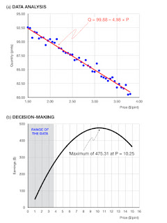
No, I haven't given up blogging; it's just on hold, while  I'm writing a short book putting together some thoughts on what people do wrong with numbers, data, and models. It'll have a lot of pictures and be priced to move.

It'll include material from some blog posts and executive education materials, reworked a bit, of course, but there's a lot of extra work involved.

Here are some of the pictures, work in progress (as usual, click for bigger):

(Adapted from this blog post.)

 (Adapted from exec-ed materials, not a blog post.)

(Adapted from this blog post.)

(Adapted from this blog post.)

Live long and prosper,

JCS

- - - - - -

Yes, the greeting is a paraphrase of the title of an AC Clarke book of collected essays.  Call it a homage.