Hidden factor correlation

Correlation is not causation; everyone learns to say that. But if there's a correlation, there's probably some sort of causal relationship hiding somewhere, unless it's a spurious correlation.

If two variables, $A$ and $B$ are correlated, the three simplest causal relationships are: $A$ causes $B$; $B$ causes $A$; or $A$ and $B$ are caused by an unseen factor $C$. There are many more complicated causation relationships, but these are the three basic ones.

The third case, where an unseen variable $C$ is the real source of the correlation, is what we're interested in this post. To illustrate the case let's say $C$ is a standard normal random variable, and $A$ and $B$ are noisy measures of $C$,

$ \qquad A = C + \epsilon_A$ and $ B = C + \epsilon_B$,

where the $\epsilon_i$ are drawn from a normal distribution with $\sigma_{\epsilon} = 0.05$.

To illustrate we generate 10,000 draws of $C$ and create the 10,000 $A$ and $B$ using R:

hidden_factor = rnorm(10000)
var_A_visible = hidden_factor + 0.05 * rnorm(10000)
var_B_visible = hidden_factor + 0.05 * rnorm(10000)

Now we can plot $A$ and $B$, and the correlation is obvious

And we can regress $A$ on $B$ to get the correlation and test statistics for the estimates using a linear model,

model_no_control = lm(var_A_visible~var_B_visible)
summary(model_no_control)

With the result:

Call:
lm(formula = var_A_visible ~ var_B_visible)

Residuals:
      Min        1Q    Median        3Q       Max 
-0.271466 -0.047214 -0.000861  0.047400  0.302517 

Coefficients:
               Estimate Std. Error  t value Pr(>|t|)    
(Intercept)   0.0005294  0.0007025    0.754    0.451    
var_B_visible 0.9975142  0.0006913 1442.852  < 2e-16 ***
---
Signif. codes:  0 ‘***’ 0.001 ‘**’ 0.01 ‘*’ 0.05 ‘.’ 0.1 ‘ ’ 1

Residual standard error: 0.07025 on 9998 degrees of freedom
Multiple R-squared:  0.9952, Adjusted R-squared:  0.9952 
F-statistic: 2.082e+06 on 1 and 9998 DF,  p-value: < 2.2e-16

So, both the model and the graph confirm a strong correlation ($p < 0.0001$) between $A$ and $B$. And in many real-life cases, this is used to support the idea that either $A$ causes $B$ or $B$ causes $A$.

Now we proceed to show how the hidden factor is relevant. First, let us plot the residuals, $A-C$ against $B-C$:

The apparent correlation has now disappeared. And a linear model including the hidden factor confirms this:

model_with_control = lm(var_A_visible~var_B_visible+hidden_factor)
summary(model_with_control)

With the result

Call:
lm(formula = var_A_visible ~ var_B_visible + hidden_factor)

Residuals:
     Min       1Q   Median       3Q      Max 
-0.18347 -0.03382 -0.00021  0.03410  0.17780 

Coefficients:
               Estimate Std. Error t value Pr(>|t|)    
(Intercept)   0.0007378  0.0004986   1.480    0.139    
var_B_visible 0.0004082  0.0100560   0.041    0.968    
hidden_factor 0.9997573  0.0100707  99.274  < 2e-16 ***
---
Signif. codes:  0 ‘***’ 0.001 ‘**’ 0.01 ‘*’ 0.05 ‘.’ 0.1 ‘ ’ 1

Residual standard error: 0.04985 on 9997 degrees of freedom
Multiple R-squared:  0.9976, Adjusted R-squared:  0.9976 
F-statistic: 2.072e+06 on 2 and 9997 DF,  p-value: < 2.2e-16

Hidden factors are easy to test for, as seen here, but they are not always apparent. For example, in nutrition papers there's often an hidden factor relating to how health-conscious an individual is that is more often than not causing both observables (say exercising regularly and eating salads; high correlation, but exercising doesn't cause eating salads and eating salads doesn't cause exercise).

Correlation is not causation, but generally one can find a causal relationship behind a correlation, possibly one that involves hidden factors or more complex relationships.

A statistical analysis of reviews of L.A. Finest: audience vs. critics

"If numbers are available, let's use the numbers. If all we have are opinions, let's go with mine." -- variously attributed to a number of bosses.

There's a new police procedural this season, L.A. Finest, and Rotten Tomatoes has done it again: critics and audience appear to be at loggerheads. Like with The Orville, Star Trek Discovery, and the last season of Doctor Who.

But "appear to be" is a dequantified statement. And Rotten Tomatoes has numbers; so, what can these numbers tell us?

Before they can tell us anything, we need to write our question: first in words, then as a math problem. Then we can solve the math problem and that solution gets translated into a "words" answer, but now a quantified "words" answer.

The question, which is suggested by the above numbers is:

Do the critics and the audience use similar or opposite criteria to rate this show?

One way to answer this question, which would have been feasible in the past when Rotten Tomatoes had user reviews, would be to do text analytics on the reviews themselves. But now the user reviews are gone so that's no longer possible.

Another way, a simpler and cleaner way, is to use the data above.

To simplify we'll assume that all ratings are either positive or negative, 0 or 1; there are some unobservable random factors that make some people like a show more or less, so these ratings are random variables. For a given person $i$, the probability that that person likes L.A. Finest is captured in some parameter $\theta_i$ (we don't observe that, of course), which is the probability of that person giving a positive rating.

So, our question above is whether the $\theta_i$ of the critics and the $\theta_i$ of the audience are the same or "opposed." And what is "opposed"? If $i$ and $j$ use opposite criteria, the probability that $i$ gives a 1 is the probability that $j$ gives a 0, so $\theta_i = 1-\theta_j$.

We don't have the individual parameters $\theta_i$ but we can simplify again by assuming that all variation within each group (critics or audience) is random, so we really only need two $\theta$.

We are comparing two situations, call them: hypothesis zero, $H_0$, meaning the critics and the audience use the same criteria, that is they have the same $\theta$, call it $\theta_0$; and hypothesis one, $H_1$, meaning the critics use criteria opposite to those of the audience, so if the critics $\theta$ is $\theta_1$, the audience $\theta$ is $(1-\theta_1)$.

Yes, I know, we don't have $\theta_0$ or $\theta_1$. We'll get there.

Our "words" question now becomes the following math problem: how much more likely is it that the data we observe is created by $H_1$ versus created by $H_0$, or in a formula: what is the likelihood ratio

$LR = \frac{\Pr(\mathrm{Data}| H_1)}{\Pr(\mathrm{Data}| H_0)} $?

Observation: This is different from the usual statistics test: the usual test is whether the two distributions are different; we are testing for a specific type of difference, opposition. So there are in fact three states of the world: same, opposite, and different but not opposite; we want to compare the likelihood of the first two. If same is much more likely than opposite, then we conclude 'same.' If opposite is much more likely than same, we conclude 'opposite.' If same and opposite have similar likelihoods (for some notion of 'similar' we'd have to investigate), then we conclude 'different but not opposite.'

Our data is four numbers: number of critics $N_C = 10$, number of positive reviews by critics $k_C = 1$, number of audience members $N_A = 40$, number of positive reviews by audience members $k_A = 30$.

But what about the $\theta_0$ and $\theta_1$?

This is where the lofty field of mathematics gives way to the down and dirty world of estimation. We estimate $\theta$ by maximum likelihood, and the maximum likelihood estimator for the probability of a positive outcome of a binary random variable (called a Bernoulli variable) is the sample mean.

Yep, all those words to say "use the share of 1s as the $\theta$."

Not so fast. True, for $H_0$, we use the share of ones

$\theta_0 = (k_C + k_A)/(N_C + N_A) = 31/50 = 0.62$;

but for $H_1$, we need to address the audience's $1-\theta_1$ by reverse coding the zeros and ones, in other words,

$\theta_1 = (k_C + (N_A - k_A))/(N_C + N_A) = 11/50 = 0.22$.

Yes, those two fractions are "estimation." Maximum likelihood estimation, at that.

Now that we are done with the dirty statistics, we come back to the shiny world of math, by using our estimates to solve the math problem. That requires a small bit of combinatorics and probability theory, all in a single sentence:

If each individual data point is an independent and identically distributed Bernoulli variable, the sum of these data points follows the binomial distribution.

Therefore the desired probabilities, which are joint probabilities of two binomial distributions, one for the critics, one for the audience, are

$\Pr(\mathrm{Data}| H_0) = c(N_C,k_C) (\theta_0)^{k_C} (1- \theta_0)^{N_C- k_C} \times c(N_A,k_A) (\theta_0)^{k_A} (1- \theta_0)^{N_A- k_A}$

and

$\Pr(\mathrm{Data}| H_1) = c(N_C,k_C) (\theta_1)^{k_C} (1- \theta_1)^{N_C- k_C} \times c(N_A,k_A) (1 -\theta_1)^{k_A} (\theta_1)^{N_A- k_A}$.

Replacing the symbols with the estimates and the data we get

$\Pr(\mathrm{Data}| H_0) = 3.222\times 10^{-5}$;
$\Pr(\mathrm{Data}| H_1) = 3.066\times 10^{-2}$.

We can now compute the likelihood ratio,

$LR = \frac{\Pr(\mathrm{Data}| H_1)}{\Pr(\mathrm{Data}| H_0)} = 915$,

and translate that into words to make the statement

It's 915 times more likely that critics are using criteria opposite to those of the audience than the same criteria.

Isn't that a lot more satisfying than saying they "appear to be at loggerheads"?

Some thoughts on quant interviews

Being a curmudgeonly quant, I started reacting to people who "love" science and math with simple Post-It questions like this:

(This is not a gotcha question, all you need is to apply Pythagorean theorem twice. I even picked numbers that work out well. Yes, $9 \sqrt{2}$ is a number that works out well.)

Which reminds me of quant interviews and their shortcomings.

I already wrote about what I think is the most important problem in quantitative thinking for the general public, in Innumeracy, Acalculia, or Numerophobia, which was inspired by this Sprezzaturian's post (Sprezzaturian was writing about quant interviews).


In search of quants

That was for the general public. This post is specifically about interviewing to determine quality of quantitative thinking. Which is more than just mathematical and statistical knowledge.

One way to test mathematical knowledge is to ask the same type of questions one gets in an exam, such as:

$\qquad$ Compute $\frac{\partial }{\partial x} \frac{\partial }{\partial y} \frac{2 \sin(x) - 3 \sin(y)}{\sin(x)\sin(y)}$.

Having interacted with self-appointed "analytics experts" who had trouble with basic calculus (sometimes even basic algebra), this kind of test sounds very appealing at first. But its focus in on the wrong side of the skill set.

Physicist Eric Mazur has the best example of the disconnect between being able to answer a technical question and understanding the material:

TL; DR: students can't apply Newton's third law of motion (for every action there's an equal and opposite reaction) to a simple problem (car collision), though they can all recite that selfsame third law. I wrote a post about this before.

Testing what matters

Knowledge tests should at the very least be complemented with (if not superseded by) "facility with quantitative thinking"-type questions. For example, let's say Bob is interviewing for a job and is given the following graph (and formula):

Nina, the interviewer, asks Bob to explain what the formula means and to grok the parameters.

Bob Who Recites Knowledge will say something like "it's a sine with argument $2 \pi \rho x$ multiplied by an exponential of $- \kappa x$; if you give me the data points I can use Excel Solver to fit a model to get estimates of $\rho$ and $\kappa$."

Bob Who Understands will start by calling the graph what it is: a dampened oscillation over $x$. Treating $x$ as time for exposition purposes, that makes $\rho$ a frequency in Hertz and $\kappa$ the dampening factor.

Next, Bob Who Understands says that there appear to be 5 1/4 cycles between 0 and 1, so $\hat \rho = 5.25$. Estimating $\kappa$ is a little harder, but since the first 3/4 cycle maps to an amplitude of $-0.75$, all we need is to solve two equations, first translating 3/4 cycle to the $x$ scale,

$\qquad$ $ 10.5 \,  \pi x = 1.5 \,  \pi$ or  $x= 0.14$

and then computing a dampening of $0.75$ at that point, since $\sin(3/2 \, \pi) = - 1$,

$\qquad$  $\exp(-\hat\kappa \times 0.14) = 0.75$, or $\hat \kappa = - \log(0.75)/0.14 = 2.3$

Bob Who Understands then says, "of course, these are only approximations; given the data points I can quickly fit a model in #rstats that gets better estimates, plus quality measures of those estimates."

(Nerd note: If instead of $e^{-\kappa x}$ the dampening had been $2^{-\kappa x}$, then $1/\kappa$ would be the half-life of the process; but the numbers aren't as clean with base $e$.)

This facility with approximate reasoning (and use of #rstats :-) signal something important about Bob Who Understands: he understands what the numbers mean in terms of their effects on the function; he groks the function.

Nina hires Bob Who Understands. Bonuses galore follow.

Bob Who Recites Knowledge joins a government agency, funding research based on "objective, quantitative" metrics, where he excels at memorizing the 264,482 pages of regulation defining rules for awarding grants.

Intellectual counterfeit fashionistas and the corruption of STEM and analytics

I have acquaintances who say they like classical music but never listen to it and can't tell Bach from Brahms. While this is entertaining to classical music aficionados, a similar disconnect happens in STEM and business analytics, where it has serious consequences.

I've observed many people who are always saying how important science is, who can name several recent Nobel laureates in the sciences, but can't compute the kinetic energy of a 2-ton SUV going 65MPH (766kJ), or, ironically, can't explain what the research of those Nobel laureates was about.

I know people who are always talking about Big Data™ and "the" Management Information Revolution™ (yes, they think the current one is the only one), but cannot write Bayes's formula and think that standard deviation is the same as standard error.

These are the signs of the rise of the intellectual counterfeit fashionista (ICF). The ICF wants others to consider him or her an intellectual (that's the I), up to date on the latest hottest intellectual topic (that's the F), but is not willing to do the work and the learning necessary to understand that topic (that's the C).

No matter how infuriating or entertaining an ICF can be on a personal level, their rise is a problem -- chiefly because of their effect on education, the practice of technical professions, and the general perception of STEM and analytics in society.

Education: by trying to recruit proto-ICFs into STEM/analytics, teaching institutions end up having to water down their courses, since the ICFs don't want to do the work needed for real learning. This leads to lower quality education for every student, even the non-ICFs.

In the mid-to-long term, this creates a number of credentialed ignoramuses and gives rise to the strange situation where people who hire engineers say there's a dearth of them, while engineering associations say there's a glut. I guess it depends on how you define engineer, by skills or by credentials.

Professions: the obvious effect of ICFs is the rise in average incompetence. The more pernicious effect is the destructive nature of internal politics, which always increase in organizations with large numbers of people for which appearances and narratives are more important than observable realities and hard work.

I wish nerdiness became unfashionable again, so that the ICFs moved on to corrupt something else and left STEM and analytics alone.

Can we stop talking about "manufacturing jobs"?

A lot of people worry about "manufacturing jobs," but the metric is seriously flawed.

Politicians and some financial analysts decry the decline of manufacturing jobs. There has been some decline, but the way these jobs are measured is inherently flawed, as it fails to take into account the change in managerial attitudes towards vertical integration.

Easy to see why with an example:

Ginormous Corp. makes widgets. In the 60s to mid-80s, as it went from being Bob's Homemade Widgets to Ginormous Corp., it added new facilities which had janitorial, accounting, cafeteria, legal, and other support services. All personnel in these support services counted as "manufacturing jobs."

In the mid-80s, Ginormous Corp. figured out (with a little help from Pain & Co and McQuincy & Co consultancies) that these support services were (a) not strategic and (b) internal monopolies. Part (a) meant that they could be outsourced and part (b) strongly suggested they should be outsourced. Let's say that Ginormous Corp. spun out these support services into wholly-owned subsidiaries, with no significant change in overall personnel.

So, all the personnel in janitorial, accounting, cafeteria, legal, and even some of the technical business support went from being in "manufacturing jobs" to being in "service jobs" without any change to what actually is produced and any actual job.

A metric that can change dramatically while the underlying system and processes don't change much is not a good foundation for decision-making. "Manufacturing jobs" is one such metric, as it depends on organizational decisions at least as much as on actual structural changes.

Metrics: useful only when well-understood.

Note: There are many reasons why focusing on manufacturing jobs over service jobs is a bad idea: Old Paul Krugman explains the most relevant, differential productivity increases, here.

Math in business courses: derivating + grokking

I used to start my Product Management class with a couple of business math problems like the following: let's say we use a given market research technique to measure the value of a product; call the product $i$ and the value $v(i)$. We know -- by choice of the technique -- that the probability that the customer will buy $i$ is given by

$\Pr(i) = \frac{\exp(v(i))}{1 + \exp(v(i))}$.

My question: is this an increasing or a decreasing function of the $v(i)$?

Typically this exercise divided students in three groups:

First, students who were afraid of math, were looking for easy credits, or otherwise unprepared for the work in the class. These math problems made sure students knew what they were getting into.

Second, students who could do the math, either by plug-and-chug (take derivative, check the sign) or by noticing that the formula may be written as

$\Pr(i) = \frac{1}{1 + \exp(-v(i))}$

and working the increasing/decreasing chain rule.

Third, students who had a quasi-intuitive understanding ("grok" in Heinlein's word) that probability of purchase must be an increasing function of value, otherwise these words are being misused.

Ideally we should be training business students to mix the skills of the last two groups: a fluency in basic mathematical thinking and grokking business implications.

- - - - - - -

Administrative note: Since I keep writing 4000+ word drafts for "important" posts that never see the light of blog (may see the light of Kindle single), I've decided to start posting these bite-sized thoughts.

Is Pete Fader right that Big Data doesn't imply big money?

He's right, in that Big Data doesn't necessarily lead to big money, but I think he exaggerates for pedagogical effect. Why he feels the need to do so is instructive, especially for Big Data acolytes.


Some days ago there was agitation in the Big Data sociosphere when an interview by Wharton marketing professor Peter Fader questioned the value of Big Data. In The Tech, Fader says

[The hype around Big Data] reminds me a lot of what was going on 15 years ago with CRM (customer relationship management). Back then, the idea was "Wow, we can start collecting all these different transactions and data, and then, boy, think of all the predictions we will be able to make." But ask anyone today what comes to mind when you say "CRM," and you'll hear "frustration," "disaster," "expensive," and "out of control." It turned out to be a great big IT wild-goose chase. And I'm afraid we're heading down the same road with Big Data. [Emphasis added.]

I think Pete's big point is correct, that Big Data by itself (to be understood as: including the computer science and the data analysis tools, not just the data -- hence the capitalization of "Big Data") is not sufficient for Big Money. I think that he's underestimating, for pedagogical effect, the role that Big Data with the application of appropriate business knowledge can have in changing the way we do marketing and the sources of value for customers (that is both the job of marketer and the foundations of business).

This is something I've blogged about before.

So, why make a point that seems fairly obvious (domain knowledge is important, not just data processing skills), and especially why make it so pointedly in a field that is full of strong personalities?

First, since a lot of people working in Big Data don't know technical marketing, they keep reinventing and rediscovering old techniques. Not only is this a duplication of work, it also ignores all knowledge of these techniques' limitations, which has been developed by marketers.

As an example of marketing knowledge that keeps being reinvented, Pete talks about the discovery of Recency-Frequency-Money in direct marketing,

The "R" part is the most interesting, because it wasn't obvious that recency, or the time of the last transaction, should even belong in the triumvirate of key measures, much less be first on the list.*    [...]

Some of those old models are really phenomenal, even today. Ask anyone in direct marketing about RFM, and they'll say, "Tell me something I don't know." But ask anyone in e-commerce, and they probably won't know what you're talking about. Or they will use a lot of Big Data and end up rediscovering the RFM wheel—and that wheel might not run quite as smoothly as the original one.

Second, some of the more famous applications of machine learning, for example the Netflix prize and computers beating humans at chess, in fact corroborate the importance of field-specific knowledge. (In other words, that which many Big Data advocates seem to believe is not important, at least as far as marketing is concerned.)

Deep Blue, the specialized chess-playing computer that defeated Kasparov, had large chess-specific pattern-matching and evaluation modules; and as for the Netflix prize, I think Isomorphismes's comment says all:

The winning BellKor/Pragmatic Chaos teams implemented ensemble methods with something like 112 techniques smushed together. You know how many of those the Netflix team implemented? Exactly two: RBM’s and SVD.    [...] 

Domain knowledge trumps statistical sophistication. This has always been the case in the recommendation engines I’ve done for clients. We spend most of our time trying to understand the space of your customers’ preferences — the cells, the topology, the metric, common-sense bounds, and so on.

Third, many people who don't know any technical marketing tools continuously disparage marketing (and its professionals), and some do so from positions of authority and leadership. That disparagement, repeated and amplified by me-too retweets and Quora upvotes, is what makes reasonable people feel the need for pointedly making their points.

Here are two paraphrased tweets by people in the Big Data sociosphere; I paraphrased them so that the authors cannot be identified with a simple search, because my objective is not to attack them but rather illustrate a more widespread attitude:

It's time marketing stopped being based on ZIP codes. (Tweeted by a principal in an analytics firm.)

Someone should write a paper on how what matters to marketing is behavior not demographics. (Tweeted by someone who writes good posts on other topics.)

To anyone who knows basic marketing, these tweets are like a kid telling a professional pianist that "we need to start playing piano with all fingers, not just the index fingers" and "it's possible to play things other than 'chopsticks' on the piano." (Both demographics and ZIP codes have been superseded by better targeting approaches many decades ago.)

These tweets reflect a sadly common attitude of Big Data people trained in computer science or statistics: that the field of marketing cannot possibly be serious, since it's not computer science or statistics. This attitude in turn extends to each of these fields: many computer scientists dismiss statistics as something irrelevant given enough data and many statisticians dismiss computer scientists as just programmers.

That's a pernicious attitude: that what has been known by others isn't worth of consideration, because we have a shiny new tool. That attitude needs deflating and that's what Pete's piece does.

-- -- -- --

* An explanation of the importance of recency is that it's a proxy  for "this client is still in a relationship with our firm." There's a paper by Schmittlein, Morrison, and Colombo, "Counting your customers," Management Science, v33n1 (1987), that develops a model of market activity using a two-state model:  the purchases are Poisson with unknown $\lambda$ in one of the states (active) and there's an unobserved probability of switching to the other state (inactive), which is absorbing and has no purchases. Under some reasonable assumptions, they show that recency increases the probability that the consumer is in the active state. BTW, I'm pretty sure that it was Pete Fader who told me about this paper, about ten years or so ago.

Analysis of the Tweets vs. Likes at the Monkey Cage

I find the question of what posts are more likely to be tweeted than liked a little strange; ideally one would want more of both.

The story so far:  a Monkey Cage post proposed some hypotheses for what characteristics of a post made it more likely to be tweeted than liked. Causal Loop did the analysis (linked at the Monkey Cage) using a composite index. Laudable as the analysis was (and how different Political Science is from the 1990s), I think I can improve upon it.

First, there are 51 (of 860 total) posts with zero likes and zero tweets. This is important information: these are posts that no one thought worthy of social media attention. Unlike Causal Loop, I want to keep these data in my dataset.

Second, instead of a ratio of likes to tweets (or more precisely, an index based on a modified ratio), I'll estimate separate models for likes and tweets, with comparable specifications. To see the problem with ratios consider the following three posts

Post A: 4 tweets, 2 likes
Post B: 8 tweets, 2 likes
Post C: 400 tweets, 200 likes

A ratio metric treats posts A and C as identical, while separating them from post B. But intuitively we expect a post like C, which generates a lot of social media activity in aggregate, to be different from posts A and B, which don't. (This scale insensitivity is a general characteristic of ratio measures.) This is one of the reasons I prefer disaggregate models. Another reason is that adding Google "+1"s would be trivial to a disaggregate model -- just run the same specifications for another dependent variable -- and complex to a ratio-based index.

To test various hypotheses one can use appropriate tests on the coefficients of the independent variables in the models or simulations to test inferences when the specifications are different (and a Hausman-like test isn't conveniently available). That's what I would do for more serious testing. With identical specifications one can compare the z-values, of course, but that's a little too reductive.

Since the likes and tweets are count variables, all that is necessary is to model the processes generating each as the aggregation of discrete events. For this post I assumed a Poisson process; its limitations are discussed below.

I loaded Causal Loop's data into Stata (yes, I could have done it in R, but since the data is in Stata format and I still own Stata, I minimized effort) and run a series of nested Poisson models: first with only the basic descriptor variables (length, graphics, video, grade level), then adding the indicator variables for the authors, then adding the indicator variables for the topics.  The all-variables-included models results (click for bigger):

A few important observations regarding this choice of models:

1. First and foremost, I'm violating the Prime Directive of model-building: I'm unfamiliar with the data. I read the Monkey Cage regularly, so I have an idea of what the posts are, but I didn't explore the data to make sure I understood what each variable meant or what the possible instantiations were. In other words, I acted as a blind data-miner. Never do this! Before building models always make sure you understand what the data mean. My excuse is that I'm not going to take the recommendations seriously and this is a way to pass the morning on Saturday. But even so, if you're one of my students, do what I say, not what I just did.

2. The choice of Poisson process as basis for the count model, convenient as it is, is probably wrong. There's almost surely state dependence in liking and tweeting: if a post is tweeted, then a larger audience (Twitter followers of the person tweeting rather than Monkey Cage readers) gets exposed to it, increasing the probability of other tweets (and also of likes -- generated from the diffusion on Twitter which brings people to the Monkey Cage who then like posts to Facebook). By using Poisson, I'm implicitly assuming a zero-order process and independence between tweets and likes -- which is almost surely not true.

3. I think including the zeros is very important. But my choice of a non-switching model implies that the differences between zero and other number of likes and tweets is only a difference of degree. It is possible, indeed likely, that they are differences of kind or process. To capture this, I'd have to build a switching model, where the determinants of zero likes or tweets were allowed to be separate from the determinants of the number of tweets and likes conditional on their being nonzero.

With all these provisos, here are some possible tongue-in-cheek conclusions from the above models:

• Joshua Tucker doesn’t influence tweetability, but his authorship decreases likability; ditto for Andrew Gelman and John Sides. Sorry, guys.
• James Fearon writes tweetable but not likable content.
• Potpourri is the least tweetable tag and also not likable; International relations is the most tweetable but not likable; Frivolity, on the other hand is highly likable. That says something about Facebook, no? 
• Newsletters are tweetable but not likable… again Nerds on Tweeter, Airheads on Facebook.

As for Joshua Tucker's hypotheses, I find some support for them, from examining the models, but I wouldn't want to commit to a support or reject before running some more elaborate tests.

Given my violation of the Prime Directive of model building (make sure you understand the data before you start building models), I wouldn't start docking the -- I'm sure -- lavish pay and benefits afforded by the Monkey Cage to its bloggers based on the numbers above.

Quantitative thinking: not for everyone. And that's bad.

Not all smart people are quantitative thinkers.

I've noticed that some smart people I know have different views of the world. Not just social, cultural, political, or aesthetic. They really do see the world through different conceptual lenses: mine are quantitative, theirs are qualitative.

Let's keep in mind that these are smart people who, when prompted to do so, can do basic math. But many of them think about the world in general, and most problems in particular, in a dequantified manner or limit their quantitative thinking in ways that don't match their knowledge of math.

Level 1 - Three different categories for quantities

Many people seem to hold the the three-level view of numbers: all quantities are divided into three bins: zero, one, many. In a previous post I explain why it's important to drill down into these categories: putting numbers in context requires, first of all, that the numbers are actual numbers, not categorical placeholders.

This tripartite view of the world is particularly bad when applied to probabilistic reasoning, because the world then becomes a three-part proposition: 0 (never), 50-50 (uncertain, which is almost always treated as the maximum entropy case), or 1 (always).

Once, at a conference, I was talking to a colleague from a prestigious school who, despite agreeing that a probability of 0.5 is different from a probability of 0.95, proceeded to argue his point based on an unstated 50-50 assumption. Knowing that $0.5 \neq 0.95$ didn't have any impact in his tripartite view of the world of uncertainty.

The problem with having a discussion with someone who thinks in terms of {zero, one, many} is that almost everything worth discussing requires better granularity than that. But the person who thinks thusly doesn't understand that it is even a problem.



Level 2 - Numbers and rudimentary statistics

Once we're past categorical thinking, things become more interesting to quantitatively focused people; this, by the way, is where a lot of muddled reasoning enters the picture. After all, many colleagues at this level of thinking believe that, by going beyond the three-category view of numbers, they are "great quants," which only proves the Dunning-Krueger effect applies.

For illustration we consider the relationship between two variables, $x$ and $y$, say depth of promotional cut (as a percentage of price) and promotional lift (as a percentage increase in unit sales due to promotion). Yep, a business example; could be politics or any social science (or science for that matter), but business is a neutral field.

At the crudest level, understanding the relationship between $x$ and $y$ can be reduced to determining whether that relationship exists at all; usually this is done by determining whether variation in one, $x$, can predict variation in the other, $y$.  For example, a company could run a contrast experiment ("A-B test" for those who believe Google invented experiments) by having half their stores run a promotion and half not; the data would then be, say:

Sales in stores without promotion: 200,000 units/store
Sales in stores with promotion: 250,000 units/store

Looks like a relationship, right? An apparent 25-percent lift (without knowing the depth of the price cut I can't comment on whether this is good or bad). But what if the average sales for all stores when there are no promotions on any store is 240,000 units/store? All this promotion apparently did was discourage some customers in the stores without promotions (the customers know about the promotion in other stores because you cannot stop information for diffusing over social media, for example) and incentivize a few of the discouraged to look for the stores running the promotion.

(A lot of anecdotes used to support public policy make the sort of mistake I just illustrated. There are plenty of other mistakes, too.)

To go beyond the simple observation of numbers and to use statistical tests, we need to have some formulation of the relationship, for example a linear one such as:

$\qquad y = \beta \, x + \epsilon$.

This formulation includes a term $\epsilon$ (called stochastic disturbance) which is the modeler's admission that we don't know everything we'd like to. (All tests have an underlying structure, even non-parametric tests; when people say that there's no structure what they are really saying is that they don't understand how the test works.)

Given some pairs of observations $\{(x_1,y_1), (x_2,y_2),\ldots\}$ , the relationship can be tested by estimating the parameter $\beta$ and determining whether the estimate $\hat \beta$ is significantly different from zero. If it's not, that means that the value of $y$ is statistically independent of $x$ (to the level of the test) and there is no relationship between them -- as far as statistical significance is concerned.

There's a lot to argue about significance testing, some of which I put in this video:

Once we get past simple tables and possibly the prepackaged statistical tests that can be done on these tables -- almost like an incantation with statistical software taking the place of the magical forces--, few people remain who want to discuss details. But even within that small set, there are many different sub-levels of thinking.



Level 3 - Thinking in models and functions

Let's go back to the linear formulation in $y = \beta \, x + \epsilon$. What this means is that lift $y$ increases with price cut $x$ in a proportional way, independent of the magnitudes of each.

Ok, so what? ask a lot of people whose level of numerical reasoning is being stretched. The "what" is that the effect of a change of price cut from 4 to 5 percent is assumed to be equal to that effect of the change from 45 to 46 percent. And this assumption is probably not true (actually, empirically we have evidence that this is not true).

Many people are able to repeat the rationale in the previous paragraph, but don't grok the implications.

The questions of where we go from this simple model are complicated. Let us ignore questions of causality for now, and focus on how different people want perceive the importance of details in the relationship between $x$ and $y$.

Increasing vs decreasing. Almost everyone who gets to this level of thinking cares about the direction of the effect. At this stage, however, many people forget that functions may be monotonic (increasing or decreasing) over an interval while outside that interval they may become non-monotonic (for example, increasing until a given point and then decreasing).

Convex versus concave. Even when the function is monotonic over the interesting domain, there's a big difference between linear, convex, and concave functions. Some disagreements with very smart people turned out to be over different assumptions regarding this second derivative: implicitly many people act as if the world is either linear or concave (assuming that the effect of adding 1 to 10 is bigger than the effect of adding 1 to 1000). As I pointed out in this post about network topologies and this post about models, combinatorics has a way of creating convexities. There's also a lot of s-shaped relationships in the world, but we'll leave those alone for now.

Functional form. As I illustrated in my post on long tails, two decreasing convex functions (the probability mass functions of the Poisson and Zipf distributions) can have very important differences. Empirical researchers are likely to care more about this than theoretical modelers, but once we reach the stage where we are discussing in these terms (and the group of people who can follow and participate in this discussion) arguments tend to be solved by mathematical inference or model calibration. In other words, leaving personal issues and inconvenient implications aside.

(Needless to say -- but I'll write it anyway -- this is the level of discussion I'd like to have when consequences are important. Alas, it's not very common; certainly not in the political or social sciences arena. In business and economics it's becoming more common and in STEM it's a foundation.)

Elaboration is still possible. I'll illustrate by noting that underlying assumptions (that I never made explicit, mind you) can come back to bite us in the gluteus maximus.

(Non-trivial statistics geekdom follows; skip till after the next picture to avoid some technical points about model building.)

Let's assume that we collect and store the data disaggregate by customer, so that $y_i$ is the quantity (not lift) bought by customer $i$; after all, we can always make aggregate data from disaggregate data but seldom can do the opposite. How would we analyze this data?

First observation: expenditures per customer are greater than zero, always. But our model might predict, for some values of $\epsilon$ a negative prediction for $y_i$  times price (which is a positive number). So our model needs to be tweaked to take into account the hard bound at zero.

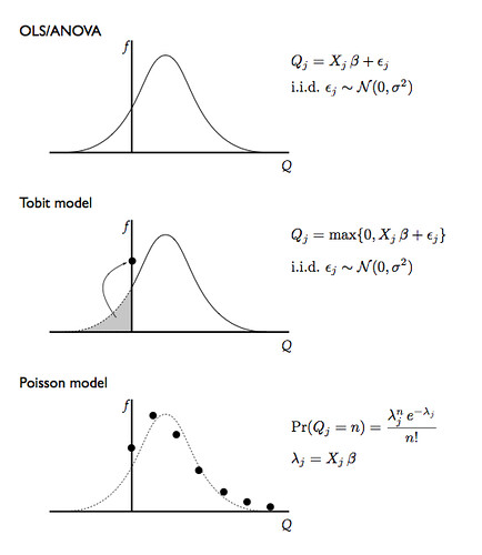
If ours were retail stores, where the data collected by the PoS scanners is only available for customers who buy something (in other words, we don't observe $y$ when $y=0$), we would have to use a technique called a censored regression; if we observe the zeros (like on a online retail site), then a model called Tobit will account for the pooling of the probability mass at zero.

Second observation: the number of units bought by any given customer is an integer; we keep treating it as a continuous quantity. Typically regression models and their variants like censored regression and Tobit assume that the stochastic disturbances are Normal variables. That would lead to possible $y_i = 1.35$, which is nonsensical in our new data: $y_i \in \{0,1,2,3,\ldots\}$.

Counting models, like a Poisson regression (which has its own assumptions) take the discreteness into account and correct the problems introduced by the continuity assumption. In olden days (when? the 50s?) these were hard models to estimate but now they are commonly included in statistical packages so there is no reason not to use them.

For illustration, here's what these models look like:

Conclusion - why is it so hard to explain these things?

Thinking quantitatively is like a super-power: where others know of phenomena, we know how much of a phenomenon.*

The problem is that this is not like a amplifier super-power, like telescopic vision is to vision, but rather an orthogonal super-power, like the ability to create multiple instances of oneself. It's hard to explain to people without the super-power (people who don't think in numbers, even though they're smart) and it's hard to understand their point of view.

Contrary to the tagline of the television show Numb3rs, not everyone thinks in numbers.

That's a pity.


-- -- -- --
* A tip of the hat to Dilbert creator Scott Adams, via Ilkka Kokkarinen's blog for pointing this out in a post which is now the opening chapter of his book.

A tale of two long tails

Power law (Zipf) long tails versus exponential (Poisson) long tails: mathematical musings with important real-world implications.

There's a lot of talk about long tails, both in finance (where fat tails, a/k/a kurtosis, turn hedging strategies into a false sense of safety) and in retail (where some people think they just invented niche marketing). I leave finance for people with better salaries brainpower, and focus only on retail for my examples.

A lot of money can be made serving the customers on the long tail; that much we already knew from decades of niche marketing. The question is how much, and for this there are quite a few considerations; I will focus on the difference between exponential decay (Poisson) long tails and hyperbolic decay (power law) long tails and how that difference would impact different emphasis on long tail targeting (that is, how much to invest going after these niche customers), say for a bookstore.

A Poisson distribution over $N\ge 0$ with parameter $\lambda$ has pdf:

$ \Pr(N=n|\lambda) =\frac{\lambda^{n}\, e^{-\lambda}}{n!}$.

A discrete power law (Zipf) distribution for $N\ge 1$ with parameter $s$ is given by:

$ \Pr(N=n|s) =\frac{n^{-s}}{\zeta(s)},$

where $\zeta(s)$ is the Riemann zeta function; note that it's only a scaling factor given $s$.

A couple of observations:

1. Because the power law has $\Pr(N=0|s)=0$, I'll actually use a Poisson + 1 process for the exponential long tail. This essentially means that the analysis would be restricted to people who buy at least one book. This assumption is not as bad as it might seem: (a) for brick-and-mortar retailers, this data is only collected when there's an actual purchase; (b) the process of buying a book at all -- which includes going to the store -- may be different from the process of deciding whether to buy a given book or the number of books to buy.

2. Since I'm not calibrating the parameters of these distributions on client data (which is confidential), I'm going to set these parameters to equalize the means of the two long tails. There are other approaches, for example setting them to minimize a measure of distance, say the Kullback-Leibler divergence or the mean square error, but the equal means is simpler.

The following diagram compares a Zipf distribution with $s=3$ (which makes $\mu=1.37$) and a 1 + Poisson process with $\lambda=0.37$ (click for larger):

The important data is the grey line, which maps into the right-side logarithmic scale: for all the visually impressive differences in the small numbers $N$ on the left, the really large ratios happen in the long tail. This is one of the issues a lot of probabilists point out to practitioners: it's really important to understand the behavior at the small probability areas of the distribution support, especially if they represent -- say -- the possibility of catastrophic losses in finance or the potential for the customers who buy large numbers of books.

An aside, from Seth Godin, about the importance of the heavy user segment in bookstores:

Amazon and the Kindle have killed the bookstore. Why? Because people who buy 100 or 300 books a year are gone forever. The typical American buys just one book a year for pleasure. Those people are meaningless to a bookstore. It's the heavy users that matter, and now officially, as 2009 ends, they have abandoned the bookstore. It's over.

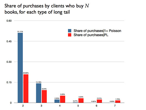
To illustrate the importance of even the relatively small ratios for a few books, this diagram shows the percentage of purchases categorized by size of purchase:

Yes, the large number of customers who buy a small number of books still gets a large percent of the total, but each of these is not a good customer to have: elaborating on Seth's post, these one-book customers are costly to serve, typically will buy a heavily-discounted best-seller and are unlikely to buy the high-margin specialized books, and tend to be followers, not influencers of what other customers will spend money on (so there are no spillovers from their purchase).

The small probabilities have been ignored long enough; finance is now becoming weary of kurtosis, marketing should go back to its roots and merge niche marketing with big data, instead of trying to reinvent the well-know wheel.

Lunchtime addendum: The differences between the exponential and the power law long tail are reproduced, to a smaller extent, across different power law regimes:

Note that the logarithmic scale implies that the increasing vertical distances with $N$ are in fact increasing probability ratios.

- - - - - - - - -

Well, that plan to make this blog more popular really panned out, didn't it? :-)

Powerful problems with power law estimation papers

Perhaps I shouldn't try to make resolutions: I resolved to blog book notes till the end of the year, and instead I'm writing something about estimation.

A power law is a relationship of the form $y = \gamma_0 x^{\gamma_1}$ and can be linearized for estimation using OLS (with a very stretchy assumption on stochastic disturbances, but let's not quibble) into

$\log(y) = \beta_0 + \beta_1 \log(x) +\epsilon$,

from which the original parameters can be trivially recovered:

$\hat\gamma_0 = \exp(\hat\beta_0)$ and $\hat\gamma_1 = \hat\beta_1$.

Power laws are plentiful in Nature, especially when one includes the degree distribution of social networks in a – generous and uncommon, I admit it – definition of Nature. An usually proposed source of power law degree distribution is preferential attachment in network formation: the probability of a new node $i$ being connected to an old node $j$ is an increasing function of the degree of $j$.

The problem with power laws in the wild is that they are really hard to estimate precisely, and I got very annoyed at the glibness of some articles, which report estimation of power laws in highly dequantized manner: they don't actually show the estimates or their descriptive statistics, only charts with no error bars.

Here's my problem: it's well-known that even small stochastic disturbances can make parameter identification in power law data very difficult. And yet, that is never mentioned in those papers. This omission, coupled with the lack of actual estimates and their descriptive statistics, is unforgivable. And suspicious.

Perhaps this needs a couple of numerical examples to clarify; as they say at the end of each season of television shows now:

– To be continued –

Data cleaning or cherry-picking?

Sometimes there's a fine line between data cleaning and cherry-picking your data.

My new favorite example of this is based on something Nassim Nicholas Taleb said at a talk at Penn (starting at 32 minutes in): that 92% of all kurtosis for silver in the last 40 years of trading could be traced to a single day; 83% of stock market kurtosis could also be traced to one day in 40 years.

One day in forty years is about 1/14,600 of all data. Such a disproportionate effect  might lead some "outlier hunters" to discard that one data point. After all, there are many data butchers (not scientists if they do this) who create arbitrary rules for outlier detection (say, more than four standard deviations away from the mean) and use them without thinking.

In the NNT case, however, that would be counterproductive: the whole point of measuring kurtosis (or, in his argument, the problem that kurtosis is not measurable in any practical way) is to hedge against risk correctly. Underestimating kurtosis will create ineffective hedges, so disposing of the "outlier" will undermine the whole point of the estimation.

In a recent research project I removed one data point from the analysis, deeming it an outlier. But I didn't do it because it was four standard deviations from the mean alone. I found it because it did show an aggregate behavior that was five standard deviations higher than the mean. Then I examined the disaggregate data and confirmed that this was anomalous behavior: the experimental subject had clicked several times on links and immediately clicked back, not even looking at the linked page. This temporally disaggregate behavior, not the aggregate measure of total clicks, was the reason why I deemed the datum an outlier, and excluded it from analysis.

Data cleaning is an important step in data analysis. We should take care to ensure that it's done correctly.

A simple, often overlooked, problem with models

There are just too many possibilities.

Let's say we have one dependent variable, $y$, and ten independent variables, $x_1,\ldots,x_{10}$. How many models can we build? For simplicity let's keep our formulation linear (in the usual sense of the word, that is linear in the coefficients; see footnote).

Inexcusably wrong answer: 11 models.

Wrong answer: 1024 models.

Right-ish answer: $1.8 \times 10^{308}$ models.

Right answer: an infinity of models.

Ok, 1024 is the number of models which include at most one instance of each variable and no interaction. Something like

$ y = \beta_0 + \beta_1 \, x_1 +  \beta_3 \, x_3 + \beta_7 \, x_7$ ,

of which there are $2^{10}$ models. (Since the constant $\beta_0$ can be zero by calibration, we'll include it in all models -- otherwise we'd have to demean the $y$.)

Once we consider possible interactions among variables, like $x_1 x_7 x_8$ for example, a three-way interaction, there are $2^{10}$ variables and interactions and therefore $2^{2^{10}}= 1.8 \times 10^{308}$ possible models with all interactions. For comparison, the number of atoms in the known universe is estimated to be in the order of $10^{80}$.

Of course, each variable can enter the model in a variety of functional forms: $x_1^{2}$, $\log(x_7)$, $\sin(5 \, x_9)$ or $x_3^{-x_{2}/2}$, for example, making it an infinite number of possibilities. (And there can be interactions between these different functions of different variables, obviously.)

(Added on August 11th.) Using polynomial approximations for generalized functions, say to the fourth degree, the total number of interactions is now $5^{10}=9765625$, as any variable may enter an interaction in one of five orders (0 through 4), and the total number of models is $2^{5^{10}}$ or around $10^{3255000}$. (End of addition.)

So here's a combinatorial riddle for statisticians: how can you identify a model out of, let's be generous, $1.8 \times 10^{308}$ with data in the exa- or petabyte range? That's almost three hundred orders of magnitude too little, methinks.

The main point is that any non-trivial set of variables can be modeled in a vast number of ways, which means that a limited number of models presented for appreciation (or review) necessarily includes an inordinate amount of judgement from the model-builder.

It's unavoidable, but seldom acknowledged.

--------------

The "linear in coefficients" point is the following. Take the following formulation, which is clearly non-linear in the $x$:

$y = \beta_0 + \beta_1 \, x_1^{1/4} + \beta_2 \, x_1 \, x_7$

but can be made linear very easily by making two changes of variables: $ z_1 =  x_1^{1/4}$ and $z_2 =  x_1 \, x_7$.

In contrast, the model $y = \alpha \, \sin( \omega \, t )$ cannot be linearized in coefficients $\alpha$ and $\omega$.

That 81% prediction, it looks good, but needs further elaboration

Bobbing around the interwebs today we find a post about a prediction of UBL's location. A tip of the homburg to Drew Conway for being the first mention I saw. Now, for the prediction itself.

As impressive as a 81% chance attributed to the actual location of UBL is, it raises three questions. These are important questions for any prediction system after its prediction is realized. Bear in mind that I'm not criticizing the actual prediction model, just the attitude of cheering for the probability without further details.

Yes, 81% is impressive; did the model make other predictions (say the location of weapons caches), and if so were they also congruent with facts? Often models will predict several variables and get some right and others wrong. Other predicted variables can act as quality control and validation. (Choice modelers typically use a hold-out sample to validate calibrated models.) It's hard to validate a model based on a single prediction.

Equally important is the size of the space of possibilities relative to the size of the predicted event. If the space was over the entire world, and the prediction pointed to Abbottabad but not Islamabad, that's impressive; if the space was restricted to Af/Pk and the model predicted the entire Islamabad district, that's a lot less impressive. I predict that somewhere in San Francisco there's a panhandler with a "Why lie, the money's for beer" poster; that's not an impressive prediction. If I predict that the panhandler is on the Market - Valencia intersection, that's impressive.

Selection is the last issue: was this the only location model for UBL or were there hundreds of competing models and we're just seeing the best? In that case it's less impressive that a model gave a high probability to the actual outcome: it's sampling on the dependent variable. For example, when throwing four dice once, getting 1-1-1-1 is very unlikely ($1/6^4 \approx 0.0008$); when throwing four dice 10 000 times, it's very likely that the 1-1-1-1 combination will appear in one of them (that probability is $1-(1- 1/6^4)^{10000} \approx 1$).

Rules of model building and inference are not there because statisticians need a barrier to entry to keep the profession profitable. (Though they sure help with paying the bills.) They are there because there's a lot of ways in which one can make wrong inferences from good models.

Usama Bin Laden had to be somewhere; a sufficiently large set of models with large enough isoprobability areas will almost surely contain a model that gives a high probability to the actual location where UBL was, especially if it was allowed to predict the location of the top hundred Al-Qaeda people and it just happened to be right about UBL.

Lessons: 1) the value of a predicted probability $\Pr(x)$ for a known event $x$ can only be understood with the context of the predicted probabilities $\Pr(y)$ for other known events $y$; 2) we must be very careful in defining what $x$ is and what the space $\mathcal{X}: x \in \mathcal{X}$ is; 3) when analyzing the results of a model, one needs to control for the existence of other models [cough] Bayesian thinking [/cough].

Effective model building and evaluation need to take into account the effects of limited reasoning by those reporting model results, or, in simpler terms, make sure you look behind the curtain before you trust the magic model to be actually magical.

Summary of this post: in acrostic!

The illusion of understanding cause and effect in complex systems

Also know as the "you're probably firing the wrong person" effect.

Consider the following market share evolution model (which is a very bad model for many reasons, and not one that should be considered for any practical application):

(1) $s[t+1] = 4 s[t] (1-s[t])$

where $s[t]$ is the share at a given time period and $s[t+1]$ is the share in the next period. This is a very bad model for market share evolution, but I can make up a story to back it up, like so:

"When this product's market share increases, there are two forces at work: first, there's imitation (the $s[t]$ part) from those who want to fit it; second there's exclusivity (the $1-s[t]$ part) from those who want to be different from the crowd. Combining these into an equation and adding a scaling factor for shares to be in the 0-1 interval, we get equation (1)."

In younger days I used to tell this story as the set-up and only point out the model's problems after the entire exercise. In case you've missed my mention, this is a very bad model of market share evolution. (See below.)

Using the model in equation (1), and starting from a market share of 75%, we notice that this is an incredibly stable market:

(2)  $s[t+1] = 4 \times 0.75 \times 0.25 = 0.75$.

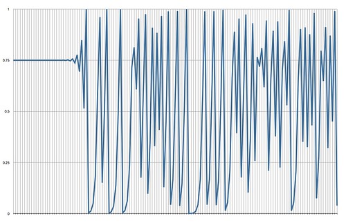
Now, what happens if instead of a market share of 75%, we start with a market share of 75.00000001%? Yes, a $10^{-10}$ precision error. Then the market share evolution is that of this graph (click for bigger):


The point of this graph is not to show that the model is ridiculous, though it does get that point across quickly, but rather to set up the following question:

When did things start to go wrong?

When I run this exercise, about 95% of the students think the answer is somewhere around period 30 (when the big oscillations begin). Then I ask why and they point out the oscillations. But there is no change in the system at period 30; in fact, the system, once primed with $s[1]=0.7500000001$, runs without change.

The problem starts at period 1. Not 30. And the lesson, which about 5% of the class gets right without my having to explain it, is that the fact that a change becomes big and visible at time $T$ doesn't mean that the cause of that change is proximate and must have happened near $T$, say at $T-1$ or $T-2$.

In complex systems, very faraway causes may create perturbations long after people have forgotten the original cause. And as is for temporal cases, like this example, so it is for spatial cases.

A lesson many managers and pundits have yet to learn.

-- -- -- -- -- -- -- -- --

The most obvious reason why this is a bad model, from the viewpoint of a manager, is that it doesn't have managerial control variables, which means that if the model were to work, the value of that manager to the company would be nil. It also doesn't work empirically or make sense logically.

Why asymmetric dominance demonstrates preference inconsistency and spoils market research tools

(Another old CB handout LaTeXed into the blog.)

Recall from the example of ``The Economist'' [in Dan Ariely's Predictably Irrational] that the options to choose from are

$A$: paper-only for 125
$B$: internet only for 65
$C$: paper + internet for 125

When presented with a choice set $\{B,C\}$ about half of the subjects pick $B$; when presented with choice set $\{A,B,C\}$ almost all subjects pick $C$. This presents a logic problem, since if C is better than B then there is no reason why it's not chosen when A is not present; if B is better than C, then there is no reason why C is chosen when A is present.

Logic is not our problem.

The reason we care about ``rational'' models is that they are the foundation of market research tools we like. In particular, we like one called utility. The idea is that we can assign numbers to choice options in a way that these numbers summarize choices (sounds like conjoint analysis, doesn't it?). Once we have these numbers we can decompose them along the dimensions of the options (yep, conjoint analysis!) and use the decomposition to determine trade-offs among products. We denote the number assigned to choice $X$ by $u(X)$.

As long as there is one number * that is assigned to each choice option by itself, we can use utility theory to analyze actual choices and determine what the drivers of customer decisions are. One number per option. Consumers facing a number of options pick that which has the highest number; this is called ``utility maximization,'' is extremely misunderstood by the general public, politicians, and the media, and all it means is that the customers choose the option they like the best, as captured by their consistent choices.

That is the problem.

Suppose we observe $B$ chosen from $\{B,C\}$; then utility theory says $u(B) > u(C)$. But then, if we observe $C$ picked from $\{A,B,C\}$ we have to conclude $u(C) > u(B)$. There are no numbers that can fit both cases at the same time, so there is no utility function. No utility function means no conjoint, no choice model, no market research --- unless we account for asymmetric dominance itself, which requires a lot of technical expertise. And forget about simple trade-off methods.

Meaning what?

Suppose we want to ignore the mathematical impossibility of coming up with a utility function (who cares about economics anyway?) and decide to measure the part-worths by hook or by crook. So we divide the products in their constituent parts, in this case $p$ for paper and $i$ for internet.  The options become $\{(p,125), (i,65),(p+i,125)\}$. We can try to make a disaggregate estimation of the part-worths using a conjoint/tradeoff model.

The problem persists.

If $(i,65)$ is chosen over $(p+i,125)$, that means that the part-worth of $p$ is less than 60. That is the conclusion we can get from the choice of $B$ from $\{B,C\}$. If $(p+i,125)$ is chosen over $(i,65)$, that means that the part-worth of $p$ is more than 60. That is the conclusion we can get from the choice of $C$ from $\{A,B,C\}$.

A marketer using these two observations to design an offering cannot determine the part-worth of one of the components: the $p$ part. It's above 60 and under 60 at the same time.

Oops.

-- -- -- -- -- -- -- -- --
* Up to any increasing transformation of the utility function numbers, if you want to get technical; we don't, and it doesn't matter anyway.

Quants make good scapegoats

Inspired by this post by Eric Falkenstein, here's some advice to managers:

You need a quant. If there's any risk you'll make a mistake, and if your boss, board, or stockholders are dumb enough to accept a pass-the-bucket excuse, you need a quant!

Quants make good scapegoats. Nobody likes smart people, nobody understands their elaborate models, and everybody wants to beat up the kids whose success is based on being smart and knowing difficult technical stuff.

You may be thinking finance is the only field blessed with such great flak-catcher posts as "Chief Economist" and "Head of Analytics," but if you're in marketing or strategy, quants are now available to you as the whipping boys for the ignorant to feed upon.

Forgot that marketing is about creating and delivering value to customers, first and foremost? (Oh, you were texting during that MBA class?) No problem, for only a zillion of your stockholders' dollars you can buy a CRM system that will support your multiple decisions to force churn the bottom 10% of customers -- until there's no one left. Then you don't need to bother with the pesky customers and can blame SAP/SAS/Accenture/Whomever. Never mind that these CRM purveyors tried hard to explain what you were doing wrong; they'll take the blame because they can't succeed by attacking their clients. At least they understand this.

No time for strategic thought? Why bother with complicated things like understanding the sources of differential advantage or identifying potential threats? You can get always a quadruple-PhD's macro-economic model to take the blame when you miss out subtle indicators, such as your competitor buying your only distribution channel. Odds are that your golfing buddies... I mean your board will side with you over the kid who can't tell a mashie from a niblick.

Don't like your quants' recommendations? Ignore them. Got in trouble? Point the finger at the nearest quant. Odds are that when quants start explaining nobody will listen, anyway. Nobody ever wants to listen to knowledgeable smart people. And the quants will be on the defensive, with only the truth on their side... and truth is so overrated in these post-modern times.

Get a quant! They're cheap insurance against your incompetence.

Because not everyone may notice this is sarcasm, my position on the above is summarized by the chyron with which I finish all my modeling classes:

Unlike the managers who blindly trust them, computer models cannot be fired.

Designers and decision-makers

I understand why Douglas Bowman is upset, but he's ultimately wrong: he makes a common error, that of using zero as an approximation for a very small number.

First, let me avoid misunderstandings: design is important and trained graphic designers tend to do it better than other people; experiments don't solve all problems and sometimes mislead managers; judgment and data complement each other. On to why Mr. Bowman is wrong, using an hypothetical based on one of his examples.

We learn that Google tested 41 different shades of blue for some clickthrough application. Given his writing, he appears to think that the idea is ridiculous; I disagree. Suppose his choice of blue is off by a very small amount; to be precise say that his favorite color leads to one in ten thousand fewer clicks than the one that does best in the experiment. (How finely tuned would his color sense have to be in order to predict a difference of 0.0001 clickability? Without the experiment we'd never know.)

The problem is that a small number in day-to-day terms (one in ten thousand) is not used in day-to-day applications (serving millions of search queries per day). Googling the number of links served per day I get about 200 million searches, each with a few sponsored links. Let's say 5 links per search, for a total of 1 billion links. Even if the average payment to Google for a clickthrough is only 5c, the difference in colors is worth $ \$5,000$ a day or 1.8 million a year. (These numbers are for illustration, but management at Google knows the real ones.)

This hypothetical loss of 1.8 million doesn't seem much compared to Google's total revenue but it is a pure opportunity cost of indulging the arrogance of credentialism (meaning: "as a trained designer I should overrule data"). I don't intend this as an attack on Mr Bowman, because I don't think most designers perceive the problem this way. But this is the business way of looking at the decision.

Ok, but what if he is right about the color choice? That is, what if after running the experiment the color that performs best is the one he had chosen?

Then the experiment will waste some clicks on the other colors and there's the added cost of running it and processing the data. Say it costs $\$100$k to do this. That means that if there is more than a 5.56% chance that Mr. Bowman is wrong by at least 0.0001 clickability, the cost of the experiment will pay itself off in one year.

Using numbers lets management ask Mr. Bowman a more precise question: Can you be 95% sure that the maximum error in color choice translates into fewer than 1 in 10,000 clicks lost?

The main problem here is the same as with most experience-based judgements when they encounter lots of data: they are roughly right and precisely wrong. And, while in each instance the error is very small to be noticed, multiplied across many instances it becomes a measurable opportunity cost.