The idea for this post came from a speech by Nassim Nicholas Taleb at Penn. Though the video is a bit rambling, it contains several important points. One that is particularly interesting to me is the difficulty of estimating the probability of rare events.
For illustration, let's consider a Normally distributed random variable $P$, and see what happens when small model errors are introduced. In particular we want to how the probability density $f_{P}(\cdot)$ predicted by four different models changes as a function of distance to zero, $x$. The higher the $x$ the more infrequently the event $P = x$ happens.
The densities are computed in the following table (click for larger):
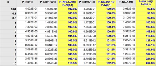
The first column gives $f_{P}(x)$ for $P \sim \mathcal{N}(0,1)$, the base case. The next column is similar except that there's a 0.1% increase in the variance (10 basis points*). The third column is the ratio of these densities. (These are not probabilities, since $P$ is a continuous variable.)
Two observations jump at us:
1. Near the mean, where most events happen, it's very difficult to separate the two cases: the ratio of the densities up to two standard deviations ($x=2$) is very close to 1.
2. Away from the mean, where events are infrequent (but potentially with high impact), the small error of 10 basis points is multiplied: at highly infrequent events ($x>7$) the density is off by over 500 basis points.
So: it's very difficult to tell the models apart with most data, but they make very different predictions for uncommon events. If these events are important when they happen, say a stock market crash, this means trouble.
Moving on, the fourth column uses $P \sim \mathcal{N}(0.001,1)$, the same 10 basis points error, but in the mean rather than the variance. Column five is the ratio of these densities to the base case.
Comparing column five with column three we see that similarly sized errors in mean estimation have less impact than errors in variance estimation. Unfortunately variance is harder to estimate accurately than the mean (it uses the mean estimate as an input, for one), so this only tells us that problems are likely to happen where they are more damaging to model predictive abilities.
Column six shows the effect of a larger variance (100 basis points off the standard, instead of 10); column seven shows the ratio of this density to the base case.
With an error of 1% in the estimate of the variance it's still hard to separate the models within two standard deviations (for a Normal distribution about 95% of all events fall within two standard deviations of the mean), but the error in density estimates at $x=7$ is 62%.
Small probability events are very hard to predict because most of the times all the information available is not enough to choose between models that have very close parameters but these models predict very different things for infrequent cases.
Told you it was a downer.
-- -- --
* Some time ago I read a criticism of this nomenclature by someone who couldn't see its purpose. The purpose is good communication design: when there's a lot of 0.01% and 0.1% being spoken in a noisy environment it's a good idea to say "one basis point" or "ten basis points" instead of "point zero one" or "zero point zero one" or "point zero zero one." It's the same reason we say "Foxtrot Universe Bravo Alpha Romeo" instead of "eff u bee a arr" in audio communication.
NOTE for probabilists appalled at my use of $P$ in $f_{P}(x)$ instead of more traditional nomenclature $f_{X}(x)$ where the uppercase $X$ would mean the variable and the lowercase $x$ the value: most people get confused when they see something like $p=\Pr(x=X)$.